Patient-Level Prediction Guide
Introduction & Purpose
Patient-Level Prediction (PLP) studies are designed to build a “risk calculator” that can predict an individual patient’s probability of experiencing a future health outcome. Unlike comparative cohort studies that estimate an average effect for a population, PLP models provide a personalised risk score for a single patient based on their unique clinical history.
The purpose of PLP is to support proactive clinical decision-making. By identifying high-risk individuals before an event occurs, clinicians can intervene earlier with preventative treatments or increased monitoring. The central question is: “Based on a patient’s baseline characteristics, can we accurately predict who is at highest risk of a future outcome?”
Study Design
The design is a prognostic model development and validation study. It involves the following key steps:
- Defining the Prediction Problem: Clearly specifying the target population, the outcome to be predicted, and the time window for the prediction.
- Feature Engineering: Extracting a large number of potential predictor variables (covariates) from the patient’s historical data.
- Model Training: Applying machine learning algorithms to a “training” dataset to learn the relationship between the baseline features and the future outcome.
- Model Validation: Evaluating the performance of the trained model on a separate “testing” dataset to ensure it is accurate and generalisable.
Participants
The study starts with a target cohort of individuals for whom we want to make a prediction (e.g., “patients newly diagnosed with diabetes”). Within this cohort, the model will be trained on individuals who have sufficient observation time to determine if they experience the outcome.
Exposures / Predictors
There is no single “exposure.” Instead, the model uses a vast number of predictor variables (also called features or covariates) extracted from the patient’s history before the prediction start date. These can include:
- Demographics
- All prior medical diagnoses
- All prior drug exposures
- All prior medical procedures
- Data from lab tests or measurements
Outcomes
The outcome is the event we are trying to predict. It must be a binary (yes/no) event that occurs within a pre-specified time-at-risk window. For example, a prediction problem could be defined as:
- Target Cohort: Patients newly diagnosed with atrial fibrillation.
- Outcome: Ischemic stroke.
- Time-at-Risk: Within 1 year after the diagnosis of atrial fibrillation.
Follow-up
Each patient in the target cohort is followed from their index date (the start of the prediction window) until either the outcome occurs, or the time-at-risk window ends.
Analyses
The analysis involves applying various machine learning algorithms to the data. The OHDSI PLP framework is designed to make this a standardised process. Key steps include:
- Data Splitting: The data is split into a training set (used to build the model) and a testing set (used to evaluate it).
- Model Training: Common algorithms used include Logistic Regression, Gradient Boosting Machines, and Random Forest. The model learns the optimal weights for each predictor variable.
- Performance Evaluation: The model’s performance is assessed on the testing set using metrics like:
- Discrimination: How well the model separates those who have the outcome from those who do not (measured by the Area Under the Receiver Operating Characteristic Curve, or AUC).
- Calibration: How well the model’s predicted probabilities match the observed reality.
The final output is a validated prediction model that can be applied to new patients to generate a personalised risk score.
How to Implement This Study
Patient-Level Prediction (PLP) aims to develop and validate prognostic models that estimate an individual patient’s probability of experiencing a future clinical outcome within a defined time-at-risk (TAR) window based on baseline health history.
How Patient-Level Prediction Works
- Target Cohort ($T$): Patients at the moment of prediction (e.g. at treatment initiation).
- Outcome Cohort ($O$): The incident binary event to predict within the Time-at-Risk (e.g. Day 1 to 365 post-index).
- Feature Engineering: Demographics and historical diagnoses extracted using
PatientProfiles. - Validation: Independent train/test splitting (
rsample), model training, discrimination assessment (ROC AUC viayardstick), and calibration evaluation.
Step 1: Setup & Connect to GiBleed
Load the necessary libraries and connect to the Eunomia GiBleed dataset using DuckDB:
library(CDMConnector)
library(CohortConstructor)
library(PatientProfiles)
library(rsample)
library(yardstick)
library(ggplot2)
library(gt)
library(dplyr)
# Connect to Eunomia GiBleed dataset
Sys.setenv(EUNOMIA_DATA_FOLDER = Sys.getenv("EUNOMIA_DATA_FOLDER", tempdir()))
if (!eunomiaIsAvailable("GiBleed")) {
  downloadEunomiaData("GiBleed")
}
##
## Download completed!
con <- DBI::dbConnect(duckdb::duckdb(), eunomiaDir("GiBleed"))
cdm <- cdmFromCon(con, cdmSchema = "main", writeSchema = "main")
Step 2: Define Target and Outcome Cohorts
We define the target population as new users of NSAIDs (Celecoxib 1118084 or Diclofenac 1124300) with at least 365 days of prior observation, and the prediction outcome as incident Gastrointestinal Hemorrhage (192671):
# 1. Target Cohort (T): Incident NSAID users
cdm$target <- conceptCohort(
  cdm = cdm,
  conceptSet = list(nsaid_users = c(1118084L, 1124300L)),
  name = "target"
) |>
  requireIsFirstEntry() |>
  requirePriorObservation(minPriorObservation = 365)

# 2. Outcome Cohort (O): Gastrointestinal Hemorrhage
cdm$outcome <- conceptCohort(
  cdm = cdm,
  conceptSet = list(gi_bleed = 192671L),
  name = "outcome"
)
Step 3: Feature Extraction & Outcome Flagging
We extract demographic variables, baseline comorbidities in the 365-day lookback window ($[-365, 0]$ days), and label whether the outcome occurred during the Time-at-Risk ($[+1, +365]$ days post-index):
# Extract baseline predictors and outcome status in Time-at-Risk (1-365 days)
features_df <- cdm$target |>
  addAge() |>
  addSex() |>
  addPriorObservation() |>
  addConceptIntersectFlag(
    conceptSet = list(
      sinusitis = 4283893L,
      uti = 4116491L,
      asthma = 4051466L
    ),
    window = c(-365, 0)
  ) |>
  addCohortIntersectFlag(
    targetCohortTable = "outcome",
    window = c(1, 365),
    nameStyle = "outcome"
  ) |>
  collect()
Step 4: Model Training and Testing
We partition the dataset into a 75% training set and a 25% testing set using stratified sampling, train a logistic regression risk model, and evaluate test-set performance:
# Prepare data for modeling
set.seed(42)
features_df$outcome_fac <- factor(
  ifelse(features_df$outcome == 1, "Event", "NoEvent"),
  levels = c("Event", "NoEvent")
)

# 75/25 Train-Test Split
split <- initial_split(features_df, prop = 0.75, strata = outcome_fac)
train_df <- training(split)
test_df <- testing(split)

# Fit prognostic risk model
model <- glm(
  outcome ~ age + sex + prior_observation + sinusitis_m365_to_0 + uti_m365_to_0 + asthma_m365_to_0,
  data = train_df,
  family = binomial()
)

# Generate test set predictions
test_df$pred_prob <- predict(model, newdata = test_df, type = "response")
test_df$pred_class <- factor(
  ifelse(test_df$pred_prob >= 0.18, "Event", "NoEvent"),
  levels = c("Event", "NoEvent")
)

# Compute ROC AUC
auc_val <- roc_auc(test_df, truth = outcome_fac, pred_prob, event_level = "first")
Step 5: Discrimination ROC Curve & Performance Summary
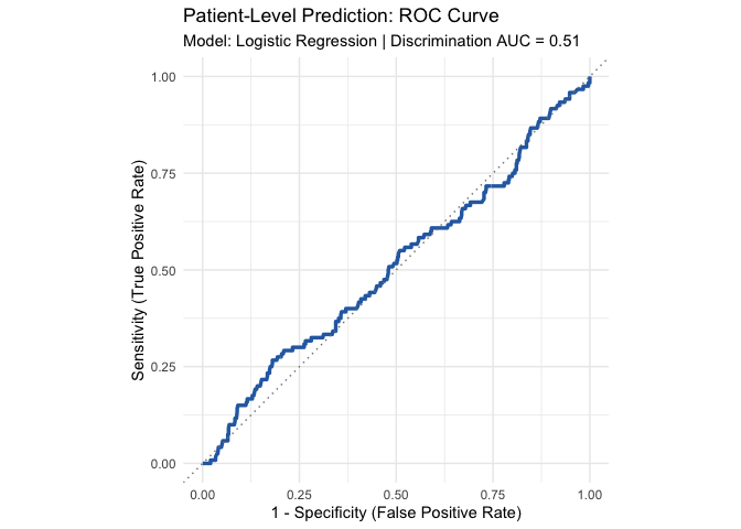
We plot the Receiver Operating Characteristic (ROC) curve and generate a publication-ready performance table:
# Generate ROC Curve
roc_df <- roc_curve(test_df, truth = outcome_fac, pred_prob, event_level = "first")

ggplot(roc_df, aes(x = 1 - specificity, y = sensitivity)) +
  geom_path(color = "#2b6cb0", linewidth = 1.2) +
  geom_abline(lty = 3, color = "grey50") +
  coord_equal() +
  labs(
    title = "Patient-Level Prediction: ROC Curve",
    subtitle = paste0("Model: Logistic Regression | Discrimination AUC = ", round(auc_val$.estimate, 3)),
    x = "1 - Specificity (False Positive Rate)",
    y = "Sensitivity (True Positive Rate)"
  ) +
  theme_minimal()
# Performance metric summary table
perf_df <- data.frame(
  Metric = c("ROC AUC (Discrimination)", "Accuracy", "Sensitivity", "Specificity"),
  Estimate = c(
    round(auc_val$.estimate, 3),
    round(accuracy(test_df, truth = outcome_fac, estimate = pred_class)$.estimate, 3),
    round(sens(test_df, truth = outcome_fac, estimate = pred_class, event_level = "first")$.estimate, 3),
    round(spec(test_df, truth = outcome_fac, estimate = pred_class, event_level = "first")$.estimate, 3)
  )
)

perf_df |>
  gt() |>
  tab_header(
    title = "Model Performance Metrics",
    subtitle = "Internal Validation on 25% Holdout Test Set"
  ) |>
  cols_label(
    Metric = "Performance Metric",
    Estimate = "Test Estimate"
  )
| Model Performance Metrics | |
| Internal Validation on 25% Holdout Test Set | |
| Performance Metric | Test Estimate |
|---|---|
| ROC AUC (Discrimination) | 0.510 |
| Accuracy | 0.503 |
| Sensitivity | 0.542 |
| Specificity | 0.494 |