R Programming Basics
This guide introduces the fundamentals of R programming, focusing on data manipulation with the tidyverse, particularly dplyr. These basics are essential before diving into OMOP-specific analyses.
Who is this guide for?
This guide is written for anyone who wants to work with databases in a “tidyverse” style—a human-centered, consistent, and composable approach to data analysis.
- New to R? We recommend complementing this guide with R for Data Science.
- New to databases? Familiarize yourself with SQL basics through tutorials like SQLBolt or SQLZoo.
- New to the OMOP CDM? This guide is best paired with The Book of OHDSI.
Bridging the Gap for Different Backgrounds
This guide is designed to be accessible to readers from various backgrounds. Here’s how we address common challenges:
For SAS Programmers
If you’re coming from SAS, you might find the functional programming style of R unfamiliar. Here’s a quick mapping of common SAS concepts to their R/dplyr equivalents:
| SAS Concept | R/dplyr Equivalent | Description |
|---|---|---|
PROC SQL | dplyr verbs like filter(), select(), mutate() | Querying and manipulating data |
DATA step | mutate() or transmute() | Creating or modifying variables |
PROC SORT | arrange() | Sorting data |
PROC SUMMARY | group_by() + summarise() | Grouping and aggregating data |
PROC FREQ | count() | Frequency tables |
Remember, in R, operations are chained using the pipe (|>) for readability, similar to how you might chain procedures in SAS.
For Clinical Experts
If you’re new to data analysis but have a strong clinical background, the OMOP CDM might seem overly complex at first. Think of it as a standardized “language” for health data:
- Why separate tables? Instead of one big spreadsheet, data is split into logical tables (e.g.,
personfor demographics,condition_occurrencefor diagnoses) to avoid repetition and ensure consistency. - What are concept IDs? These are standardized codes for medical terms (e.g., “Type 2 Diabetes” might have ID 201826). They ensure everyone uses the same definitions, making research comparable.
- Why vocabularies? OMOP uses controlled vocabularies (like SNOMED or ICD) to map local codes to standard ones, reducing ambiguity.
This structure allows for powerful, scalable analyses across different healthcare systems.
For Data Scientists New to Healthcare (like Martina)
If you’re proficient in R but unfamiliar with clinical research, we’ll explain the “why” behind the code. For example, when we create a “cohort” of patients, it’s not just filtering data—it’s defining a study population based on clinical criteria to answer specific research questions.
How is this guide organized?
This guide is divided into two main parts:
- General Principles for Working with Databases in R: The first half focuses on the foundational concepts of using tidyverse-style code to build analytical pipelines. You will learn how to connect to a database, manipulate data, and prepare it for analysis without ever leaving the R environment.
- Applying these Principles to the OMOP CDM: The second half demonstrates how to apply these general principles specifically to the OMOP Common Data Model. We will explore a suite of specialized R packages that streamline common analytical tasks in observational health research.
Detailed Chapters Overview
For a deeper dive, the underlying technical manual for this guide is structured into the following detailed chapters. While this page provides a high-level summary, the full manual offers comprehensive examples and technical explanations.
1. A first analysis using data in a database
The iris dataset is a classic example in data science, collected by Edgar Anderson in 1935. It contains measurements of 150 iris flowers from three species: setosa, versicolor, and virginica. Each flower has four measurements: sepal length, sepal width, petal length, and petal width (all in centimeters). The goal is often to classify the species based on these measurements, making it a simple but effective dataset for demonstrating statistical and machine learning techniques.
Setting Up Your Environment
First, you need to install and load the necessary R packages.
# Load the libraries
library(dplyr)
library(dbplyr)
library(ggplot2)
library(DBI)
library(duckdb)
Inserting Data into a Database
Next, we will load the iris data into an in-memory duckdb database. This simulates a real-world scenario where your data resides in a database server.
# Create an in-memory duckdb database
db <- dbConnect(drv = duckdb())

# Write the iris dataframe to a table named "iris" in the database
dbWriteTable(db, "iris", iris)

# You can see the tables in the database
dbListTables(db)
## [1] "iris"
# > [1] "iris"
From R to SQL: The Power of dbplyr
Now that the data is in a database, we could query it using SQL. However, the magic of the dbplyr package is that it allows you to write familiar dplyr code, which it automatically translates into SQL for you.
First, create a reference to the iris table in the database.
iris_db <- tbl(db, "iris")
Now, you can use standard dplyr verbs on this object.
# Get a summary of sepal length by species
iris_db |>
  group_by(Species) |>
  summarise(
    n = n(),
    mean_sepal_length = mean(Sepal.Length, na.rm = TRUE)
  )
## # Source:   SQL [?? x 3]
## # Database: DuckDB 1.4.0 [gabriel.maeztu@Darwin 25.0.0:R 4.5.1/:memory:]
##   Species        n mean_sepal_length
##   <fct>      <dbl>             <dbl>
## 1 setosa        50              5.01
## 2 versicolor    50              5.94
## 3 virginica     50              6.59
When you run this code, dbplyr translates it into the following SQL query, sends it to the database, and returns the result.
<SQL>
SELECT
  "Species",
  COUNT(*) AS n,
  AVG("Sepal.Length") AS mean_sepal_length
FROM iris
GROUP BY "Species"
Bringing Data into R for Visualization
While most data manipulation should happen in the database for efficiency, you will often need to bring the final, summarized data back into R for visualization or modeling. The collect() function does this.
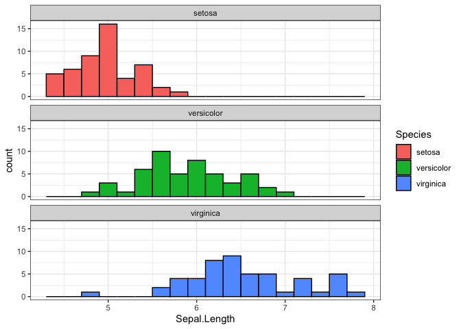
Let’s create a histogram of sepal length for each flower species.
iris_db |>
  select("Species", "Sepal.Length") |>
  collect() |> # This brings the data from the database into an R dataframe
  ggplot(aes(x = `Sepal.Length`, fill = Species)) +
  geom_histogram(binwidth = 0.2, colour = "black") +
  facet_wrap(~Species, ncol = 1) +
  theme_bw()
This workflow—manipulating data in the database and collecting only the results—is the most efficient way to work with large datasets.
Disconnecting from the Database
When you are finished with your analysis, it is good practice to close the connection to the database.
dbDisconnect(db)
2. Core verbs for analytic pipelines utilising a database
To demonstrate working with multiple tables, we’ll extend the iris example by creating related tables. We’ll split the data into separate tables for species information and measurements, then show how to join them back together.
Setting Up the Database with Multiple Tables
# Create database
db <- dbConnect(duckdb())

# Split iris into two tables: species info and measurements
species_info <- iris |> select(Species) |> distinct() |> mutate(species_id = row_number())
measurements <- iris |> left_join(species_info, by = "Species")

# Write tables
dbWriteTable(db, "species_info", species_info)
dbWriteTable(db, "measurements", measurements)

# Create lazy references
species_db <- tbl(db, "species_info")
measurements_db <- tbl(db, "measurements")
Selecting Rows: filter() and distinct()
Use filter() to select rows based on conditions. For example, to find measurements with sepal length > 5:
measurements_db |>
  filter(Sepal.Length > 5) |>
  select(Species, Sepal.Length)
## # Source:   SQL [?? x 2]
## # Database: DuckDB 1.4.0 [gabriel.maeztu@Darwin 25.0.0:R 4.5.1/:memory:]
##    Species Sepal.Length
##    <fct>          <dbl>
##  1 setosa           5.1
##  2 setosa           5.4
##  3 setosa           5.4
##  4 setosa           5.8
##  5 setosa           5.7
##  6 setosa           5.4
##  7 setosa           5.1
##  8 setosa           5.7
##  9 setosa           5.1
## 10 setosa           5.4
## # ℹ more rows
distinct() removes duplicate rows:
measurements_db |>
  distinct(Species)
## # Source:   SQL [?? x 1]
## # Database: DuckDB 1.4.0 [gabriel.maeztu@Darwin 25.0.0:R 4.5.1/:memory:]
##   Species
##   <fct>
## 1 setosa
## 2 virginica
## 3 versicolor
Ordering Rows: arrange()
arrange() sorts rows by one or more columns:
measurements_db |>
  arrange(desc(Sepal.Length)) |>
  select(Species, Sepal.Length)
## # Source:     SQL [?? x 2]
## # Database:   DuckDB 1.4.0 [gabriel.maeztu@Darwin 25.0.0:R 4.5.1/:memory:]
## # Ordered by: desc(Sepal.Length)
##    Species   Sepal.Length
##    <fct>            <dbl>
##  1 virginica          7.9
##  2 virginica          7.7
##  3 virginica          7.7
##  4 virginica          7.7
##  5 virginica          7.7
##  6 virginica          7.6
##  7 virginica          7.4
##  8 virginica          7.3
##  9 virginica          7.2
## 10 virginica          7.2
## # ℹ more rows
Column Transformation: mutate(), select(), rename()
mutate() creates or modifies columns:
measurements_db |>
  mutate(
    sepal_ratio = Sepal.Length / Sepal.Width,
    is_large = Sepal.Length > 6
  ) |>
  select(Species, sepal_ratio, is_large)
## # Source:   SQL [?? x 3]
## # Database: DuckDB 1.4.0 [gabriel.maeztu@Darwin 25.0.0:R 4.5.1/:memory:]
##    Species sepal_ratio is_large
##    <fct>         <dbl> <lgl>
##  1 setosa         1.46 FALSE
##  2 setosa         1.63 FALSE
##  3 setosa         1.47 FALSE
##  4 setosa         1.48 FALSE
##  5 setosa         1.39 FALSE
##  6 setosa         1.38 FALSE
##  7 setosa         1.35 FALSE
##  8 setosa         1.47 FALSE
##  9 setosa         1.52 FALSE
## 10 setosa         1.58 FALSE
## # ℹ more rows
select() chooses specific columns:
measurements_db |>
  select(Species, Sepal.Length, Petal.Length)
## # Source:   SQL [?? x 3]
## # Database: DuckDB 1.4.0 [gabriel.maeztu@Darwin 25.0.0:R 4.5.1/:memory:]
##    Species Sepal.Length Petal.Length
##    <fct>          <dbl>        <dbl>
##  1 setosa           5.1          1.4
##  2 setosa           4.9          1.4
##  3 setosa           4.7          1.3
##  4 setosa           4.6          1.5
##  5 setosa           5            1.4
##  6 setosa           5.4          1.7
##  7 setosa           4.6          1.4
##  8 setosa           5            1.5
##  9 setosa           4.4          1.4
## 10 setosa           4.9          1.5
## # ℹ more rows
rename() changes column names:
measurements_db |>
  rename(sepal_length = Sepal.Length)
## # Source:   SQL [?? x 6]
## # Database: DuckDB 1.4.0 [gabriel.maeztu@Darwin 25.0.0:R 4.5.1/:memory:]
##    sepal_length Sepal.Width Petal.Length Petal.Width Species species_id
##           <dbl>       <dbl>        <dbl>       <dbl> <fct>        <int>
##  1          5.1         3.5          1.4         0.2 setosa           1
##  2          4.9         3            1.4         0.2 setosa           1
##  3          4.7         3.2          1.3         0.2 setosa           1
##  4          4.6         3.1          1.5         0.2 setosa           1
##  5          5           3.6          1.4         0.2 setosa           1
##  6          5.4         3.9          1.7         0.4 setosa           1
##  7          4.6         3.4          1.4         0.3 setosa           1
##  8          5           3.4          1.5         0.2 setosa           1
##  9          4.4         2.9          1.4         0.2 setosa           1
## 10          4.9         3.1          1.5         0.1 setosa           1
## # ℹ more rows
Grouping and Aggregation: group_by(), summarise(), count()
group_by() groups data for calculations:
measurements_db |>
  group_by(Species) |>
  summarise(
    avg_sepal = mean(Sepal.Length, na.rm = TRUE),
    count = n()
  )
## # Source:   SQL [?? x 3]
## # Database: DuckDB 1.4.0 [gabriel.maeztu@Darwin 25.0.0:R 4.5.1/:memory:]
##   Species    avg_sepal count
##   <fct>          <dbl> <dbl>
## 1 setosa          5.01    50
## 2 versicolor      5.94    50
## 3 virginica       6.59    50
count() is a shortcut for counting:
measurements_db |>
  count(Species, sort = TRUE)
## # Source:     SQL [?? x 2]
## # Database:   DuckDB 1.4.0 [gabriel.maeztu@Darwin 25.0.0:R 4.5.1/:memory:]
## # Ordered by: desc(n)
##   Species        n
##   <fct>      <dbl>
## 1 setosa        50
## 2 versicolor    50
## 3 virginica     50
Joining Tables
Joins combine data from multiple tables. For example, to join measurements with species info:
measurements_db |>
  left_join(species_db, by = "Species") |>
  select(Species, Sepal.Length)
## # Source:   SQL [?? x 2]
## # Database: DuckDB 1.4.0 [gabriel.maeztu@Darwin 25.0.0:R 4.5.1/:memory:]
##    Species Sepal.Length
##    <fct>          <dbl>
##  1 setosa           5.1
##  2 setosa           4.9
##  3 setosa           4.7
##  4 setosa           4.6
##  5 setosa           5
##  6 setosa           5.4
##  7 setosa           4.6
##  8 setosa           5
##  9 setosa           4.4
## 10 setosa           4.9
## # ℹ more rows
Constructing a Tidy Analytic Dataset
Let’s create a comprehensive dataset by joining tables and performing aggregations:
analytic_dataset <- measurements_db |>
  group_by(Species) |>
  summarise(
    avg_sepal_length = mean(Sepal.Length, na.rm = TRUE),
    avg_petal_length = mean(Petal.Length, na.rm = TRUE),
    total_measurements = n()
  ) |>
  arrange(desc(avg_sepal_length))

# Collect results
analytic_dataset |> collect()
## # A tibble: 3 × 4
##   Species    avg_sepal_length avg_petal_length total_measurements
##   <fct>                 <dbl>            <dbl>              <dbl>
## 1 virginica              6.59             5.55                 50
## 2 versicolor             5.94             4.26                 50
## 3 setosa                 5.01             1.46                 50
This pipeline demonstrates how to build complex queries using dplyr verbs, with all operations pushed to the database for efficiency.
3. Supported expressions for database queries
Data Type Conversions
R and SQL handle data types differently. dbplyr automatically converts many types, but understanding the mappings is important:
- Logical:
TRUE/FALSE→TRUE/FALSEor1/0 - Character: Strings remain strings
- Numeric: Integers and doubles are preserved
- Dates:
Dateobjects →DATE - Datetimes:
POSIXct→TIMESTAMP
Logical Comparisons and Operators
Standard comparison operators work as expected:
measurements_db |> filter(Sepal.Length > 5 & Petal.Length > 3)
## # Source:   SQL [?? x 2]
## # Database: DuckDB 1.4.0 [gabriel.maeztu@Darwin 25.0.0:R 4.5.1/:memory:]
##    Sepal.Length Sepal.Width Petal.Length Petal.Width Species    species_id
##           <dbl>       <dbl>        <dbl>       <dbl> <fct>           <int>
##  1          7           3.2          4.7         1.4 versicolor          2
##  2          6.4         3.2          4.5         1.5 versicolor          2
##  3          6.9         3.1          4.9         1.5 versicolor          2
##  4          5.5         2.3          4           1.3 versicolor          2
##  5          6.5         2.8          4.6         1.5 versicolor          2
##  6          5.7         2.8          4.5         1.3 versicolor          2
##  7          6.3         3.3          4.7         1.6 versicolor          2
##  8          6.6         2.9          4.6         1.3 versicolor          2
##  9          5.2         2.7          3.9         1.4 versicolor          2
## 10          5.9         3            4.2         1.5 versicolor          2
## # ℹ more rows
# Translates to: WHERE "Sepal.Length" > 5 AND "Petal.Length" > 3
Conditional Statements
if_else() and case_when() are supported:
measurements_db |>
  mutate(
    size_category = case_when(
      Sepal.Length < 5 ~ "small",
      Sepal.Length <= 6 ~ "medium",
      TRUE ~ "large"
    )
  )
## # Source:   SQL [?? x 7]
## # Database: DuckDB 1.4.0 [gabriel.maeztu@Darwin 25.0.0:R 4.5.1/:memory:]
##    Sepal.Length Sepal.Width Petal.Length Petal.Width Species species_id
##           <dbl>       <dbl>        <dbl>       <dbl> <fct>        <int>
##  1          5.1         3.5          1.4         0.2 setosa           1
##  2          4.9         3            1.4         0.2 setosa           1
##  3          4.7         3.2          1.3         0.2 setosa           1
##  4          4.6         3.1          1.5         0.2 setosa           1
##  5          5           3.6          1.4         0.2 setosa           1
##  6          5.4         3.9          1.7         0.4 setosa           1
##  7          4.6         3.4          1.4         0.3 setosa           1
##  8          5           3.4          1.5         0.2 setosa           1
##  9          4.4         2.9          1.4         0.2 setosa           1
## 10          4.9         3.1          1.5         0.1 setosa           1
## # ℹ more rows
## # ℹ 1 more variable: size_category <chr>
SQL translation:
CASE
  WHEN "Sepal.Length" < 5 THEN 'small'
  WHEN "Sepal.Length" <= 6 THEN 'medium'
  ELSE 'large'
END
String Functions
Common string operations:
species_db |>
  mutate(
    species_upper = toupper(Species),
    species_length = nchar(Species),
    species_substr = substr(Species, 1, 3)
  )
## # Source:   SQL [?? x 5]
## # Database: DuckDB 1.4.0 [gabriel.maeztu@Darwin 25.0.0:R 4.5.1/:memory:]
##   Species    species_id species_upper species_length species_substr
##   <fct>           <int> <chr>                  <dbl> <chr>
## 1 setosa              1 SETOSA                     6 set
## 2 versicolor          2 VERSICOLOR                10 ver
## 3 virginica           3 VIRGINICA                  9 vir ```
Database-Specific Considerations
While dbplyr aims for portability, some functions may behave differently:
- DuckDB: Full support for most R functions
- PostgreSQL: Excellent date/time support
- SQL Server: May require workarounds for some functions
Always test your queries on your target database system.
4. Building analytic pipelines for a data model
Principles of Modular Pipelines
- Separation of Concerns: Break down complex queries into smaller, focused steps
- Reusability: Create functions for common operations
- Readability: Use clear variable names and comments
- Efficiency: Minimize data movement between database and R
Example: Analyzing Iris Measurements
Building on the iris example, let’s create a pipeline to analyze measurements by species:
# Step 1: Filter and prepare data
iris_performance <- measurements_db |>
  filter(!is.na(Sepal.Length), !is.na(Petal.Length))

# Step 2: Calculate metrics
performance_metrics <- iris_performance |>
  mutate(
    sepal_petal_ratio = Sepal.Length / Petal.Length,
    is_large_flower = as.numeric(Sepal.Length > 6)
  ) |>
  group_by(Species) |>
  summarise(
    total_flowers = n(),
    avg_sepal_petal_ratio = mean(sepal_petal_ratio, na.rm = TRUE),
    large_percentage = mean(is_large_flower, na.rm = TRUE) * 100
  )

# Step 3: Filter for significant groups
significant_species <- performance_metrics |>
  filter(total_flowers >= 40) |>
  arrange(desc(avg_sepal_petal_ratio))

# Collect results
results <- significant_species |> collect()
Creating Reusable Functions
For repeated operations, create functions:
calculate_ratios <- function(measurements_tbl) {
  measurements_tbl |>
    mutate(
      sepal_petal_ratio = Sepal.Length / Petal.Length,
      is_large = as.numeric(Sepal.Length > 6)
    ) |>
    summarise(
      total = n(),
      avg_ratio = mean(sepal_petal_ratio, na.rm = TRUE),
      large_pct = mean(is_large, na.rm = TRUE)
    )
}

# Use the function
species_ratios <- measurements_db |>
  group_by(Species) |>
  calculate_ratios()
Handling Complex Joins in Relational Models
In structured data models like OMOP, you’ll often need to join multiple tables. Plan your joins carefully:
- Identify the central table (e.g.,
personin OMOP) - Determine the join keys
- Consider the join type (left, inner, etc.)
- Chain joins logically
This approach ensures your pipelines are maintainable and efficient.