Comparative Cohort Studies Guide
Introduction & Purpose
Comparative Cohort Studies are one of the most common and powerful designs in observational research. Their purpose is to emulate a clinical trial by comparing the risk of health outcomes between two or more groups of patients who have received different medical interventions. This design is the cornerstone of causal inference in real-world evidence, helping us to understand the relative safety and effectiveness of different treatments.
The central question this design answers is: “Is Treatment A associated with a higher or lower risk of an outcome than Treatment B?”
To answer this question reliably, the study must be carefully designed to minimise bias, particularly confounding by indication, which occurs when the patient groups receiving different treatments are not comparable at baseline.
Study Design
The design is a comparative cohort analysis. It involves identifying at least two distinct cohorts of patients, a target cohort (receiving the treatment of interest) and a comparator cohort (receiving an alternative treatment), and following them over time to observe the occurrence of pre-specified outcomes.
Key variations of this design include:
- New User Design: This is the preferred approach. It includes only patients who are newly initiating either the target or comparator treatment. This design avoids many biases associated with prevalent users and provides a clear “time zero” for the start of follow-up.
- Prevalent User Design: This design includes patients who are current users of the treatments. It can be necessary when studying treatments for chronic conditions where new users are rare, but it requires more complex methods to control for biases.
Participants
The study includes at least two cohorts of patients, defined by their exposure to the treatments being compared. A critical step is to define a set of inclusion and exclusion criteria to ensure the study population is appropriate for the research question. This often includes requiring a minimum period of data visibility before treatment initiation.
Exposures
The exposures are the medical interventions being compared. In a typical study, these are:
- Target Exposure: The drug or treatment of primary interest.
- Comparator Exposure: An alternative drug or treatment, often the standard of care, used as a benchmark for comparison. This is known as an active comparator design.
Outcomes
The study pre-specifies one or more health outcomes of interest. These can be safety outcomes (e.g., adverse events) or effectiveness outcomes (e.g., disease remission). To assess the validity of the study, a set of negative control outcomes (outcomes not believed to be caused by either treatment) are often included to detect residual bias.
Follow-up
For each patient, follow-up begins on the day they initiate their respective treatment (the index date). Follow-up continues until the first occurrence of:
- The outcome of interest.
- Switching to or adding the other cohort’s treatment.
- Discontinuation of the treatment (in an “on-treatment” analysis).
- Loss to follow-up or end of data availability.
Analyses
The analysis aims to estimate the causal effect of the target exposure relative to the comparator. The key analytical step is to control for confounding. This is typically done using Propensity Scores, which are the predicted probability of a patient receiving the target treatment given their baseline characteristics.
Common propensity score methods include:
- Matching: Creating pairs of similar patients from the target and comparator groups.
- Stratification: Dividing patients into strata based on their propensity score.
- Inverse Probability of Treatment Weighting (IPTW): Weighting each patient by the inverse of their propensity score.
After balancing the cohorts, the analysis involves calculating the relative risk of the outcome, often expressed as a Hazard Ratio from a Cox regression model or a Rate Ratio from a Poisson model.
How to Implement This Study
The CohortSurvival and CohortConstructor packages provide tools for executing comparative cohort time-to-event analyses within the OMOP Common Data Model.
How Comparative Cohort Survival Works
- Active Comparator Design: Define target and comparator treatment cohorts using standard OMOP concepts with
CohortConstructor. - New-User Requirement: Restrict entries to incident users with a defined lookback period (
requirePriorObservation). - Survival Estimation: Compute non-parametric Kaplan-Meier survival curves and cumulative event probabilities using
estimateSingleEventSurvival(). - Stratification & Visualisation: Generate publication tables and faceted survival plots using
tableSurvival()andplotSurvival().
Step 1: Setup & Connect to GiBleed
Load the necessary libraries and connect to the Eunomia GiBleed dataset using DuckDB:
library(CDMConnector)
library(CohortConstructor)
library(CohortSurvival)
library(visOmopResults)
library(dplyr)
# Connect to Eunomia GiBleed dataset
Sys.setenv(EUNOMIA_DATA_FOLDER = Sys.getenv("EUNOMIA_DATA_FOLDER", tempdir()))
if (!eunomiaIsAvailable("GiBleed")) {
  downloadEunomiaData("GiBleed")
}
##
## Download completed!
con <- DBI::dbConnect(duckdb::duckdb(), eunomiaDir("GiBleed"))
cdm <- cdmFromCon(con, cdmSchema = "main", writeSchema = "main")
Step 2: Build Target, Comparator, and Outcome Cohorts
We define new users of Celecoxib (concept_id = 1118084) as the target exposure, Diclofenac (concept_id = 1124300) as the active comparator exposure, and Gastrointestinal Hemorrhage (concept_id = 192671) as the safety outcome:
# 1. Instantiate Exposure Cohorts (Target & Active Comparator)
cdm$exposure <- conceptCohort(
  cdm = cdm,
  conceptSet = list(
    celecoxib = 1118084L,
    diclofenac = 1124300L
  ),
  name = "exposure"
) |>
  requireIsFirstEntry() |>
  requirePriorObservation(minPriorObservation = 365)

# 2. Instantiate Outcome Cohort (Gastrointestinal Hemorrhage)
cdm$outcome <- conceptCohort(
  cdm = cdm,
  conceptSet = list(gi_bleed = 192671L),
  name = "outcome"
)
Step 3: Estimate Time-to-Event Survival
We estimate single-event survival probability comparing the risk of gastrointestinal hemorrhage between the two treatments:
# Estimate Kaplan-Meier survival curves
surv_estimates <- estimateSingleEventSurvival(
  cdm = cdm,
  targetCohortTable = "exposure",
  outcomeCohortTable = "outcome"
)
Step 4: Display Survival Tables and Event Summaries
We generate structured summaries of survival estimates and observed outcome event counts across follow-up time:
# Summary table of survival probabilities
tableSurvival(surv_estimates, times = c(0, 30, 90, 180, 365))
| Data source | Target cohort | Outcome name | Estimate name | ||||||||
|---|---|---|---|---|---|---|---|---|---|---|---|
| Number records | Number events | Median survival (95% CI) | Restricted mean survival (95% CI) | 0 days survival estimate | 30 days survival estimate | 90 days survival estimate | 180 days survival estimate | 365 days survival estimate | |||
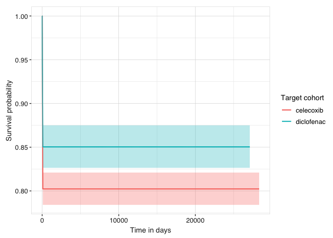
| Synthea | celecoxib | gi_bleed | 1,800 | 355 | – | 22,738.00 (22,217.00, 23,259.00) | 100.00 (100.00, 100.00) | 93.72 (92.60, 94.84) | 80.23 (78.41, 82.10) | 80.23 (78.41, 82.10) | 80.23 (78.41, 82.10) |
| diclofenac | gi_bleed | 830 | 124 | – | 23,057.00 (22,399.00, 23,714.00) | 100.00 (100.00, 100.00) | 94.46 (92.91, 96.03) | 85.03 (82.64, 87.50) | 85.03 (82.64, 87.50) | 85.03 (82.64, 87.50) | |
# Table of outcome events and person-time constrained to key milestones
surv_estimates |>
  filterAdditional(time %in% c(0, 30, 90, 180, 365)) |>
  tableSurvivalEvents()
| Data source | Target cohort | Outcome name | Time | Event gap | Estimate name | ||
|---|---|---|---|---|---|---|---|
| Number at risk | Number events | Number censored | |||||
| Synthea | celecoxib | gi_bleed | 0 | 30 | 1,800 | 0 | 0 |
| 30 | 30 | 1,688 | 113 | 3 | |||
| 90 | 30 | 1,438 | 130 | 3 | |||
| 180 | 30 | 1,431 | 0 | 4 | |||
| diclofenac | gi_bleed | 0 | 30 | 830 | 0 | 0 | |
| 30 | 30 | 783 | 46 | 1 | |||
| 90 | 30 | 703 | 39 | 1 | |||
| 180 | 30 | 700 | 0 | 3 | |||
Step 5: Plot Kaplan-Meier Curves
We visualize the comparative Kaplan-Meier curves for Celecoxib versus Diclofenac users:
# Plot comparative Kaplan-Meier survival curves
plotSurvival(surv_estimates, colour = "target_cohort")