Pathway Analysis Guide
Introduction & Purpose
Pathway Analysis is a descriptive study designed to map out the “patient journey” by discovering and visualizing the sequence of clinical events people experience over time. While the most common application is for Treatment Pathways, the same methodology can be applied to sequences of medical procedures or the progression of diagnosed conditions.
While a Drug Utilisation Study might tell you how many people used a drug, a pathway analysis tells you the order, timing, and combination in which they experienced multiple clinical events. The purpose is to understand real-world clinical practice and patient progression. This can help answer important questions such as:
- For Treatments: What is the most common first-line therapy for a disease, and what is the typical second-line therapy?
- For Procedures: What is the common sequence of surgical interventions for a condition?
- For Diseases: How does a disease typically progress from an initial diagnosis to later-stage complications?
This information is invaluable for understanding adherence to clinical guidelines, identifying common patient trajectories, and contextualising the results of other observational studies.
Study Design
The design is a descriptive cohort study focused on sequencing clinical events over time. It is a data-driven discovery process that does not involve a comparator group or traditional hypothesis testing.
Participants
The study begins with a target cohort of individuals who have a specific characteristic of interest (e.g., a new diagnosis of a disease). The analysis then focuses on tracking the occurrence of a pre-specified list of relevant clinical events (e.g., specific medications, procedures, or related diagnoses) for this cohort.
Events of Interest (Exposures)
The “exposures” are the clinical events that will be sequenced. The power of this method is its flexibility; these events can be:
- Drug Exposures: To create a treatment pathway.
- Procedure Occurrences: To create a procedural pathway.
- Condition Occurrences: To create a disease progression pathway.
The analysis tracks the initiation and timing of these different events over time.
Outcomes
The “outcomes” of this study are the discovered pathways themselves. The primary outputs are visualisations, most commonly Sankey diagrams or sunburst plots, which show the flow of patients from one event to the next. The analysis also produces summary statistics, such as:
- The proportion of patients who start on each first-line event.
- The median time between sequential events.
- The probability of transitioning from one specific event to another.
Follow-up
Follow-up for each patient begins at their cohort index date and continues until the end of data availability or a pre-defined study end date. The analysis engine tracks all occurrences of the specified clinical events during this period.
Analyses
The analysis is a descriptive, data-mining process. The key steps are:
- Event Identification: Identifying all occurrences of the events of interest for each patient in the cohort.
- Era Construction: Consolidating adjacent or overlapping events into continuous “eras.”
- Pathway Construction: Sequencing these eras chronologically for each patient to construct their individual pathway.
- Pathway Aggregation: Aggregating the individual pathways to identify the most common sequences across the entire cohort.
The final result is a quantitative and visual summary of the most frequently travelled patient journeys.
How to Implement This Study
Pathway Analysis maps out the real-world sequence, combination, and transition of therapies or clinical events experienced by patients over time following an initial disease diagnosis.
How Pathway Analysis Works
- Target Cohort: Patients diagnosed with a condition of interest establishing index “time zero”.
- Event Extraction & Era Building: Extracting subsequent drug exposures, collapsing adjacent records into treatment eras.
- Line of Therapy Assignment: Chronologically ordering treatment eras into Line 1 (L1), Line 2 (L2), and Line 3 (L3).
- Pathway Aggregation & Visualisation: Quantifying the most frequent therapeutic sequences and visualizing patient journey flows.
Step 1: Setup & Connect to GiBleed
Load the necessary libraries and establish a connection to the Eunomia GiBleed dataset using DuckDB:
library(CDMConnector)
library(CohortConstructor)
library(dplyr)
library(tidyr)
library(ggplot2)
library(gt)
# Connect to Eunomia GiBleed dataset
Sys.setenv(EUNOMIA_DATA_FOLDER = Sys.getenv("EUNOMIA_DATA_FOLDER", tempdir()))
if (!eunomiaIsAvailable("GiBleed")) {
  downloadEunomiaData("GiBleed")
}
##
## Download completed!
con <- DBI::dbConnect(duckdb::duckdb(), eunomiaDir("GiBleed"))
cdm <- cdmFromCon(con, cdmSchema = "main", writeSchema = "main")
Step 2: Define Index Diagnosis Cohort
We define our target cohort as incident patients diagnosed with Sinusitis (concept_id = 4283893, 4294548):
# Target Cohort: Incident Sinusitis Patients
cdm$sinusitis <- conceptCohort(
  cdm = cdm,
  conceptSet = list(sinusitis = c(4283893L, 4294548L)),
  name = "sinusitis"
) |>
  requireIsFirstEntry()
Step 3: Extract Longitudinal Medications & Construct Lines of Therapy
We extract all subsequent drug exposures following the diagnosis date, consolidate consecutive exposures into treatment eras, and classify each patient’s journey into sequential lines of therapy:
# Extract post-diagnosis drug exposures
drugs <- cdm$sinusitis |>
  select(person_id = subject_id, diag_date = cohort_start_date) |>
  inner_join(
    cdm$drug_exposure |> select(person_id, drug_concept_id, drug_exposure_start_date),
    by = "person_id"
  ) |>
  filter(drug_exposure_start_date >= diag_date) |>
  left_join(cdm$concept |> select(concept_id, concept_name), by = c("drug_concept_id" = "concept_id")) |>
  collect() |>
  mutate(
    treatment = case_when(
      grepl("Ampicillin", concept_name, ignore.case = TRUE) ~ "Ampicillin",
      grepl("celecoxib", concept_name, ignore.case = TRUE) ~ "Celecoxib",
      grepl("Diclofenac", concept_name, ignore.case = TRUE) ~ "Diclofenac",
      grepl("vaccine|toxoid", concept_name, ignore.case = TRUE) ~ "Vaccines",
      TRUE ~ "Other"
    )
  ) |>
  arrange(person_id, drug_exposure_start_date) |>
  group_by(person_id) |>
  mutate(prev_treatment = lag(treatment)) |>
  filter(is.na(prev_treatment) | treatment != prev_treatment) |>
  mutate(line_num = row_number()) |>
  filter(line_num <= 3) |>
  mutate(line = paste0("Line_", line_num)) |>
  ungroup()

# Pivot to patient-level pathways
pathways <- drugs |>
  pivot_wider(id_cols = person_id, names_from = line, values_from = treatment) |>
  mutate(
    Line_1 = ifelse(is.na(Line_1), "None", Line_1),
    Line_2 = ifelse(is.na(Line_2), "Discontinued", Line_2),
    Line_3 = ifelse(is.na(Line_3), "Discontinued", Line_3)
  )
Step 4: Top Treatment Pathways Summary Table
We aggregate the individual patient journeys into top treatment pathways:
# Summarise most common treatment pathways
pathway_summary <- pathways |>
  group_by(Line_1, Line_2, Line_3) |>
  summarise(Patients_N = n(), .groups = "drop") |>
  mutate(Percentage = round((Patients_N / sum(Patients_N)) * 100, 1)) |>
  arrange(desc(Patients_N)) |>
  head(10)

pathway_summary |>
  gt() |>
  tab_header(
    title = "Top Treatment Pathways Following Sinusitis Diagnosis",
    subtitle = "Sequence Progression across Lines 1, 2, and 3"
  ) |>
  cols_label(
    Line_1 = "1st Line Therapy",
    Line_2 = "2nd Line Therapy",
    Line_3 = "3rd Line Therapy",
    Patients_N = "Patients (N)",
    Percentage = "Proportion (%)"
  )
| Top Treatment Pathways Following Sinusitis Diagnosis | ||||
| Sequence Progression across Lines 1, 2, and 3 | ||||
| 1st Line Therapy | 2nd Line Therapy | 3rd Line Therapy | Patients (N) | Proportion (%) |
|---|---|---|---|---|
| Other | Vaccines | Other | 478 | 35.9 |
| Vaccines | Other | Vaccines | 169 | 12.7 |
| Other | Celecoxib | Other | 139 | 10.4 |
| Other | Celecoxib | Vaccines | 74 | 5.6 |
| Other | Vaccines | Celecoxib | 72 | 5.4 |
| Other | Diclofenac | Other | 62 | 4.7 |
| Other | Discontinued | Discontinued | 37 | 2.8 |
| Vaccines | Discontinued | Discontinued | 32 | 2.4 |
| Other | Vaccines | Discontinued | 31 | 2.3 |
| Celecoxib | Other | Vaccines | 26 | 2.0 |
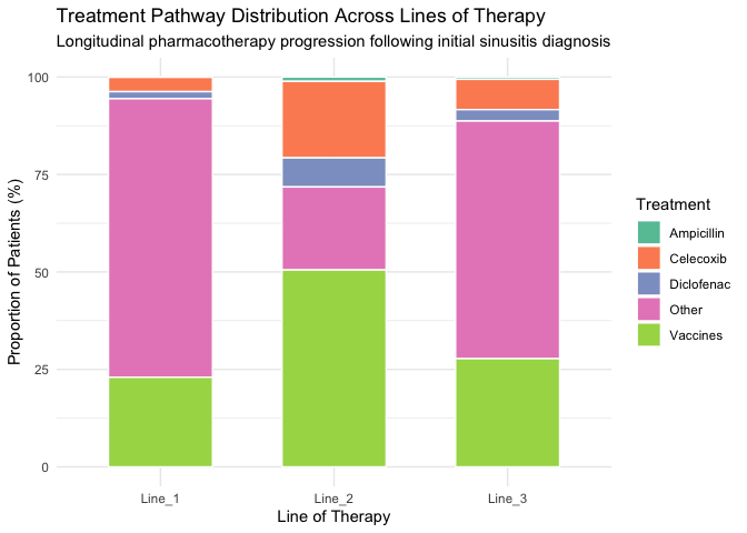
Step 5: Visualizing Treatment Flow across Lines
We plot the distribution of therapeutic modalities across successive lines of therapy:
# Aggregate by line and treatment
plot_df <- drugs |>
  group_by(line, treatment) |>
  summarise(n = n(), .groups = "drop") |>
  group_by(line) |>
  mutate(pct = (n / sum(n)) * 100)

ggplot(plot_df, aes(x = line, y = pct, fill = treatment)) +
  geom_col(position = "stack", width = 0.6, color = "white") +
  scale_fill_brewer(palette = "Set2") +
  labs(
    title = "Treatment Pathway Distribution Across Lines of Therapy",
    subtitle = "Longitudinal pharmacotherapy progression following initial sinusitis diagnosis",
    x = "Line of Therapy",
    y = "Proportion of Patients (%)",
    fill = "Treatment"
  ) +
  theme_minimal()