Population-Level Epidemiology Guide
Introduction & Purpose
Population-Level Epidemiology studies are designed to answer the most fundamental questions in public health: how common is a disease within a population, and is its frequency changing over time? This methodology provides a high-level, panoramic view of a disease’s burden on a community or healthcare system, which is essential for planning public health policies, allocating resources, and identifying emerging health trends.
The purpose is to quantify the frequency of health outcomes at a population level, typically by measuring:
- Incidence: The rate of new cases of a disease in a population over a specific period. This helps us understand the risk of developing the disease.
- Prevalence: The proportion of a population that currently has a disease at a specific point in time (point prevalence) or over a period (period prevalence). This helps us understand the overall burden of the disease.
Study Design
The standard design for this analysis is a population-level cohort study. This involves taking the entire population captured within a database and following them over a defined period of calendar time to observe the occurrence of health outcomes.
Participants
The study typically includes the entire source population available in the database who have a minimum period of data visibility (e.g., at least one year) before the study’s start date. Key considerations for defining the participant group include:
- For Incidence Calculation: To measure only new cases, individuals who have a history of the disease (prevalent cases) are excluded from the analysis. This “washout” period ensures that the cases being counted are genuinely new diagnoses.
- Subpopulations: The analysis can be restricted to specific subpopulations of interest, for example, by limiting the study to people over a certain age or with a specific clinical history.
Outcomes
The primary outcomes are the calculated rates of incidence and prevalence for the disease of interest. These are typically stratified by:
- Demographics: Age groups and gender.
- Time: Calendar year, month, or quarter to observe trends.
Follow-up
The follow-up for the study begins at a pre-defined calendar date (the index date) and continues for a specified period (e.g., one year). This process is often repeated for multiple consecutive periods to generate trend data over several years.
Analyses
The analytical approach is descriptive. The core calculations are:
- Incidence Rate: The number of newly diagnosed people (the numerator) divided by the total person-time at risk in the population (the denominator).
- Prevalence: The number of people with the diagnosis (both new and pre-existing) divided by the total number of people in the source population at a specific point in time or over a period.
How to Implement This Study
The OHDSI IncidencePrevalence R package is designed to calculate population-level incidence and prevalence rates from OMOP CDM data, directly addressing the core analytical requirements of this study design.
At a high level, IncidencePrevalence turns OMOP CDM cohorts into tidy, stratified summaries by repeatedly applying three ideas:
- Denominator time: People contribute at-risk time only when they meet the study rules you set with
generateDenominatorCohortSet()/generateTargetDenominatorCohortSet(). Entry is the latest of study start, prior observation met, and minimum age; exit is the earliest of study end, observation end, and age upper limit. - Outcome overlap: Outcomes are read from a separate cohort table you prepare (here provided by
mockIncidencePrevalence()). Prevalence checks whether a person is in the outcome cohort at a time point/over an interval; incidence counts first qualifying onsets, respecting washout and repeated event rules. - Interval slicing: The study time is cut into calendar intervals (years, quarters, months). Each interval gets its own denominator, outcome counts, and derived measures.
Key computations and arguments
- Point prevalence (
estimatePointPrevalence):- What: proportion with the outcome at a time point inside each interval.
- How: outcome presence on the chosen
timePoint(“start”/“middle”/“end”) among those in the denominator at that date. - Tip: Use when you want a snapshot at a consistent anchor within each interval.
- Period prevalence (
estimatePeriodPrevalence):- What: proportion with the outcome at any time during the interval.
- How: outcome occurs at any day overlapping the interval; denominator includes those present during the interval.
fullContribution: ifTRUE, only people observed for the entire interval count in the denominator; ifFALSE, anyone observed for ≥1 day counts.- Tip: Choose
fullContributionbased on whether incomplete observation could bias proportions for long intervals.
- Incidence (
estimateIncidence):- What: new-onset rates per person-time in each interval.
- How: counts qualifying outcome onsets and divides by person-time contributed in the denominator.
outcomeWashout: requires no outcome in the prior N days; useInfto ensure first-ever incidence.repeatedEvents: ifTRUE, allows multiple incident events per person separated by washout; ifFALSE, at most one incident event per person.completeDatabaseIntervals: ifTRUE, drops intervals where the database cannot establish full observation coverage (e.g., first/last years with partial data), reducing edge bias.
Stratification and groups
- Groups: Each combination of denominator settings (age group, sex, prior history, time-at-risk windows, target-based subsets) becomes a separate
cohort_definition_idand produces separate rows. - Strata: You can facet/colour or summarize by variables such as
denominator_age_group,denominator_sex, etc. UseplotIncidence()/plotPrevalence()helpers andavailable...Grouping()to see valid aesthetics.
Outputs
- Summarised results: Functions return a “summarised_result” tables with
estimate_name/valuepairs, plus additional metadata (start/end dates, interval type). These are directly consumable byvisOmopResultstotableIncidence/tablePrevalenceand plot functions.
Practical guidance
- Pick intervals aligned to your question and data density (years for long-term trends, months for seasonality).
- Use
outcomeWashoutandrepeatedEventsto encode “first-ever” vs. “episode-based” incidence. - Prefer
completeDatabaseIntervals(incidence) and considerfullContribution(period prevalence) when edge effects or intermittent observation could bias estimates. - Keep exclusion logic out of outcome cohorts; define restrictions on the denominator instead.
Our workflow will follow a simple, powerful pattern common across OHDSI packages: summarise -> table/plot.
Step 1: Load Libraries & Connect to the GiBleed Database
First, we load the necessary libraries. CDMConnector provides the connection to the OMOP CDM database, CohortConstructor builds clinical cohorts from standard OMOP concepts, IncidencePrevalence calculates population-level epidemiology rates, and visOmopResults formats the results into publication-ready tables and plots.
We connect to the standardized Eunomia GiBleed dataset using DuckDB:
library(CDMConnector)
library(CohortConstructor)
library(IncidencePrevalence)
library(visOmopResults)
library(dplyr)
# Ensure GiBleed dataset is available and connect via DuckDB
Sys.setenv(EUNOMIA_DATA_FOLDER = Sys.getenv("EUNOMIA_DATA_FOLDER", tempdir()))
if (!eunomiaIsAvailable("GiBleed")) {
  downloadEunomiaData("GiBleed")
}
##
## Download completed!
con <- DBI::dbConnect(duckdb::duckdb(), eunomiaDir("GiBleed"))
cdm <- cdmFromCon(con, cdmSchema = "main", writeSchema = "main")
Step 2: Define Outcome and Denominator Cohorts
In this study, our outcome of interest is Gastrointestinal Hemorrhage (concept_id = 192671). We instantiate the outcome cohort directly from the OMOP CDM condition table:
# Create the gastrointestinal hemorrhage outcome cohort
cdm$outcome <- conceptCohort(
  cdm = cdm,
  conceptSet = list(gi_bleed = 192671L),
  name = "outcome"
)
Next, we define our source study population (the denominator). We will study the population observed between 2010 and 2019, stratifying by age groups (0–49 and 50–100) and by sex:
# Define the denominator cohort for the study period
cdm <- generateDenominatorCohortSet(
  cdm = cdm,
  name = "denominator",
  cohortDateRange = as.Date(c("2010-01-01", "2019-01-01")),
  ageGroup = list(
    c(0, 49),
    c(50, 100)
  ),
  sex = c("Male", "Female")
)
Step 3: Calculate Incidence & Prevalence (The summarise Step)
This step calculates incidence and prevalence rates across the defined strata.
3.1: Estimate Incidence
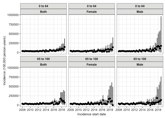
We calculate annual incidence rates for gastrointestinal hemorrhage. We set outcomeWashout = Inf to include only first-ever occurrences and repeatedEvents = FALSE. We then visualize the results with plotIncidence() and generate a structured table with tableIncidence():
# Calculate annual incidence rates
inc <- estimateIncidence(
  cdm = cdm,
  denominatorTable = "denominator",
  outcomeTable = "outcome",
  interval = "years",
  outcomeWashout = Inf,
  repeatedEvents = FALSE
)

# Plot incidence rates faceted by age group and colored by sex
plotIncidence(inc, facet = "denominator_age_group", colour = "denominator_sex")
# Display concise 5-year recent trend table
inc |>
  filterAdditional(incidence_start_date >= as.Date("2014-01-01")) |>
  tableIncidence()
| Incidence start date | Incidence end date | Denominator age group | Denominator sex | Estimate name | |||
|---|---|---|---|---|---|---|---|
| Denominator (N) | Person-years | Outcome (N) | Incidence 100,000 person-years [95% CI] | ||||
| Synthea; gi_bleed | |||||||
| 2014-01-01 | 2014-12-31 | 0 to 49 | Female | 510 | 498.47 | 6 | 1,203.68 (441.73 - 2,619.90) |
| 2015-01-01 | 2015-12-31 | 0 to 49 | Female | 487 | 469.42 | 4 | 852.12 (232.17 - 2,181.76) |
| 2016-01-01 | 2016-12-31 | 0 to 49 | Female | 450 | 433.06 | 5 | 1,154.57 (374.88 - 2,694.38) |
| 2017-01-01 | 2017-12-31 | 0 to 49 | Female | 413 | 375.99 | 8 | 2,127.72 (918.60 - 4,192.46) |
| 2018-01-01 | 2018-12-31 | 0 to 49 | Female | 324 | 237.49 | 5 | 2,105.38 (683.61 - 4,913.25) |
| 2014-01-01 | 2014-12-31 | 0 to 49 | Male | 477 | 459.10 | 3 | 653.45 (134.76 - 1,909.66) |
| 2015-01-01 | 2015-12-31 | 0 to 49 | Male | 441 | 425.36 | 8 | 1,880.75 (811.97 - 3,705.82) |
| 2016-01-01 | 2016-12-31 | 0 to 49 | Male | 410 | 390.78 | 4 | 1,023.59 (278.89 - 2,620.79) |
| 2017-01-01 | 2017-12-31 | 0 to 49 | Male | 371 | 334.98 | 9 | 2,686.76 (1,228.56 - 5,100.31) |
| 2018-01-01 | 2018-12-31 | 0 to 49 | Male | 280 | 190.53 | 5 | 2,624.26 (852.09 - 6,124.14) |
| 2014-01-01 | 2014-12-31 | 50 to 100 | Female | 583 | 573.66 | 0 | 0.00 (0.00 - 643.04) |
| 2015-01-01 | 2015-12-31 | 50 to 100 | Female | 614 | 595.25 | 0 | 0.00 (0.00 - 619.72) |
| 2016-01-01 | 2016-12-31 | 50 to 100 | Female | 635 | 622.14 | 0 | 0.00 (0.00 - 592.94) |
| 2017-01-01 | 2017-12-31 | 50 to 100 | Female | 658 | 643.15 | 0 | 0.00 (0.00 - 573.56) |
| 2018-01-01 | 2018-12-31 | 50 to 100 | Female | 674 | 591.38 | 0 | 0.00 (0.00 - 623.78) |
| 2014-01-01 | 2014-12-31 | 50 to 100 | Male | 598 | 575.42 | 0 | 0.00 (0.00 - 641.07) |
| 2015-01-01 | 2015-12-31 | 50 to 100 | Male | 610 | 595.87 | 0 | 0.00 (0.00 - 619.08) |
| 2016-01-01 | 2016-12-31 | 50 to 100 | Male | 634 | 619.35 | 0 | 0.00 (0.00 - 595.61) |
| 2017-01-01 | 2017-12-31 | 50 to 100 | Male | 656 | 638.86 | 0 | 0.00 (0.00 - 577.41) |
| 2018-01-01 | 2018-12-31 | 50 to 100 | Male | 683 | 593.91 | 0 | 0.00 (0.00 - 621.12) |
3.2: Estimate Point Prevalence
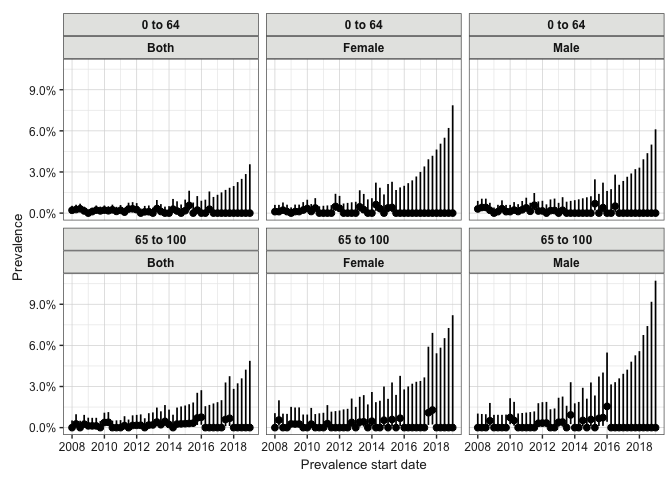
Next, we estimate annual point prevalence at the start of each year (timePoint = "start"):
# Calculate annual point prevalence
prev_point <- estimatePointPrevalence(
  cdm = cdm,
  denominatorTable = "denominator",
  outcomeTable = "outcome",
  interval = "years",
  timePoint = "start"
)

# Plot point prevalence faceted by age group and colored by sex
plotPrevalence(prev_point, facet = "denominator_age_group", colour = "denominator_sex")
# Display concise 5-year recent trend table
prev_point |>
  filterAdditional(prevalence_start_date >= as.Date("2014-01-01")) |>
  tablePrevalence()
| Prevalence start date | Prevalence end date | Denominator age group | Denominator sex | Estimate name | ||
|---|---|---|---|---|---|---|
| Denominator (N) | Outcome (N) | Prevalence [95% CI] | ||||
| Synthea; gi_bleed | ||||||
| 2014-01-01 | 2014-01-01 | 0 to 49 | Female | 581 | 0 | 0.00 (0.00 - 0.01) |
| 2015-01-01 | 2015-01-01 | 0 to 49 | Female | 554 | 0 | 0.00 (0.00 - 0.01) |
| 2016-01-01 | 2016-01-01 | 0 to 49 | Female | 516 | 0 | 0.00 (0.00 - 0.01) |
| 2017-01-01 | 2017-01-01 | 0 to 49 | Female | 475 | 0 | 0.00 (0.00 - 0.01) |
| 2018-01-01 | 2018-01-01 | 0 to 49 | Female | 377 | 0 | 0.00 (0.00 - 0.01) |
| 2019-01-01 | 2019-01-01 | 0 to 49 | Female | 156 | 0 | 0.00 (0.00 - 0.02) |
| 2014-01-01 | 2014-01-01 | 0 to 49 | Male | 549 | 0 | 0.00 (0.00 - 0.01) |
| 2015-01-01 | 2015-01-01 | 0 to 49 | Male | 510 | 0 | 0.00 (0.00 - 0.01) |
| 2016-01-01 | 2016-01-01 | 0 to 49 | Male | 480 | 0 | 0.00 (0.00 - 0.01) |
| 2017-01-01 | 2017-01-01 | 0 to 49 | Male | 442 | 0 | 0.00 (0.00 - 0.01) |
| 2018-01-01 | 2018-01-01 | 0 to 49 | Male | 338 | 0 | 0.00 (0.00 - 0.01) |
| 2019-01-01 | 2019-01-01 | 0 to 49 | Male | 127 | 0 | 0.00 (0.00 - 0.03) |
| 2014-01-01 | 2014-01-01 | 50 to 100 | Female | 683 | 0 | 0.00 (0.00 - 0.01) |
| 2015-01-01 | 2015-01-01 | 50 to 100 | Female | 708 | 0 | 0.00 (0.00 - 0.01) |
| 2016-01-01 | 2016-01-01 | 50 to 100 | Female | 739 | 0 | 0.00 (0.00 - 0.01) |
| 2017-01-01 | 2017-01-01 | 50 to 100 | Female | 770 | 0 | 0.00 (0.00 - 0.00) |
| 2018-01-01 | 2018-01-01 | 50 to 100 | Female | 798 | 0 | 0.00 (0.00 - 0.00) |
| 2019-01-01 | 2019-01-01 | 50 to 100 | Female | 482 | 0 | 0.00 (0.00 - 0.01) |
| 2014-01-01 | 2014-01-01 | 50 to 100 | Male | 681 | 0 | 0.00 (0.00 - 0.01) |
| 2015-01-01 | 2015-01-01 | 50 to 100 | Male | 707 | 0 | 0.00 (0.00 - 0.01) |
| 2016-01-01 | 2016-01-01 | 50 to 100 | Male | 730 | 0 | 0.00 (0.00 - 0.01) |
| 2017-01-01 | 2017-01-01 | 50 to 100 | Male | 756 | 0 | 0.00 (0.00 - 0.01) |
| 2018-01-01 | 2018-01-01 | 50 to 100 | Male | 783 | 0 | 0.00 (0.00 - 0.00) |
| 2019-01-01 | 2019-01-01 | 50 to 100 | Male | 456 | 0 | 0.00 (0.00 - 0.01) |