Patient-Level Characterisation Guide
Introduction & Purpose
A Patient-Level Characterisation study is the observational research equivalent of creating a “Table 1” in a clinical trial. Its primary purpose is to generate a detailed clinical and demographic profile of a specific group of patients (a cohort). This answers the fundamental question: “Who are these patients?”
This type of analysis is a cornerstone of transparent and reproducible research. By providing a comprehensive baseline description of the study population, it helps researchers and readers understand the context of the study, assess the generalisability of the findings, and identify potential sources of confounding or bias.
Study Design
The design is a descriptive cohort analysis. It focuses on summarising the characteristics of one or more cohorts of patients at a specific point in time (the index date), or within a defined time window before it.
Participants
The study includes one or more cohorts of interest. These cohorts are typically defined by a shared characteristic, such as:
- A new diagnosis of a specific condition.
- The initiation of a particular medication.
- Undergoing a specific medical procedure.
A key requirement is that participants have a period of data visibility (e.g., one year) before their index date to allow for the assessment of baseline characteristics.
Exposures / Covariates
In this context, there is no “exposure” in the comparative sense. Instead, the analysis focuses on summarising a wide range of patient covariates (characteristics) present at or before the index date. These can include:
- Demographics: Age, gender, race, ethnicity.
- Clinical History: All recorded medical conditions, often summarised into comorbidity scores like the Charlson Comorbidity Index.
- Medication History: All prior medications the patients have used.
- Procedures: A history of medical procedures.
Outcomes
The “outcomes” of this study are the summary statistics for the covariates of interest. The analysis produces tables and visualisations that describe the distribution of these characteristics within the cohort. This can include:
- For categorical variables: Frequencies and percentages (e.g., % of patients with a history of diabetes).
- For continuous variables: Means, medians, and standard deviations (e.g., mean age of the cohort).
Follow-up
There is typically no follow-up period after the index date in a pure characterisation study. The focus is entirely on the baseline period before the index date.
Analyses
The analysis is descriptive and involves summarising the covariates. This can be done in two ways:
- Large-Scale Characterisation: An automated process that summarises thousands of clinical features from the database to provide an unbiased, data-driven overview of the cohort.
- Pre-Specified Characterisation: An analysis focused on a limited set of clinically important covariates that have been defined in advance by the researchers.
The results are typically presented in a summary table, often referred to as “Table 1,” which provides a comprehensive snapshot of the cohort.
How to Implement This Study
Let’s implement the study using the OHDSI CohortCharacteristics and PatientProfiles packages to generate baseline profiles (“Table 1”) of one or more cohorts in the OMOP CDM, directly addressing the guide’s descriptive design.
How CohortCharacteristics works
- Summarise -> table/plot:
summariseCohortCount/summariseCharacteristicsproduce tidysummarised_resultoutputs consumed bytable…/plot…helpers invisOmopResults. - Cohorts in, summaries out: You provide one or more cohort tables (OMOP CDM structure). Functions compute counts, attrition, demographics, and clinical features at/before index.
- Windows: For granular baselines, large-scale summaries can use windows (e.g., -365:-1, 0:0, 1:365) around index.
- Groups/strata: Each cohort produces groups; you can stratify or facet by
cohort_nameand other variables in plots/tables.
Practical guidance
- Connect to standard benchmark datasets (such as Eunomia GiBleed) for reproducible evaluation.
- Keep cohort inclusion/exclusion logic in cohort construction; keep
summarisefunctions descriptive. - Save the
summarised_resultobject and then render tables/plots.
Step 1: Setup
This initial step focuses on preparing the R environment for the analysis. It involves loading libraries like CDMConnector, CohortConstructor, CohortCharacteristics, and PatientProfiles.
library(CDMConnector)
library(CohortConstructor)
library(CohortCharacteristics)
library(PatientProfiles)
library(visOmopResults)
library(dplyr)
Step 2: Connect to the GiBleed CDM and Create Cohorts
We connect to the standardized Eunomia GiBleed dataset using DuckDB. We define two comparative cohorts of interest—individuals exposed to Celecoxib (concept_id = 1118084) and Diclofenac (concept_id = 1124300).
# Ensure GiBleed dataset is available and connect via DuckDB
Sys.setenv(EUNOMIA_DATA_FOLDER = Sys.getenv("EUNOMIA_DATA_FOLDER", tempdir()))
if (!eunomiaIsAvailable("GiBleed")) {
  downloadEunomiaData("GiBleed")
}
##
## Download completed!
con <- DBI::dbConnect(duckdb::duckdb(), eunomiaDir("GiBleed"))
cdm <- cdmFromCon(con, cdmSchema = "main", writeSchema = "main")

# Generate cohorts for Celecoxib and Diclofenac
cdm$nsaids <- conceptCohort(
  cdm = cdm,
  conceptSet = list(
    celecoxib = 1118084L,
    diclofenac = 1124300L
  ),
  name = "nsaids"
)
Step 3: Cohort counts and attrition
Before diving into detailed characterization, it’s important to understand the size and composition of each cohort. This step calculates the number of subjects and records in each cohort and inspects the attrition process.
# Summarize the number of subjects and records in each cohort
counts <- summariseCohortCount(cdm$nsaids)
# Display the cohort counts in a table
tableCohortCount(counts)
| CDM name | Variable name | Estimate name | Cohort name | |
|---|---|---|---|---|
| celecoxib | diclofenac | |||
| Synthea | Number records | N | 1,800 | 830 |
| Number subjects | N | 1,800 | 830 | |
# Summarize the attrition of the cohorts
attr <- summariseCohortAttrition(cdm$nsaids)
# Display the cohort attrition in a table
tableCohortAttrition(attr)
| Reason | Variable name | |||
|---|---|---|---|---|
| number_records | number_subjects | excluded_records | excluded_subjects | |
| Synthea; celecoxib | ||||
| Initial qualifying events | 1,844 | 1,844 | 0 | 0 |
| Record in observation | 1,800 | 1,800 | 44 | 44 |
| Not missing record date | 1,800 | 1,800 | 0 | 0 |
| Merge overlapping records | 1,800 | 1,800 | 0 | 0 |
| Synthea; diclofenac | ||||
| Initial qualifying events | 850 | 850 | 0 | 0 |
| Record in observation | 830 | 830 | 20 | 20 |
| Not missing record date | 830 | 830 | 0 | 0 |
| Merge overlapping records | 830 | 830 | 0 | 0 |
Step 4: Baseline characteristics (“Table 1”) and plots
This is the core of the patient-level characterization analysis. We generate a comprehensive summary of baseline characteristics, often referred to as “Table 1,” describing age, sex, and prior observation time at cohort entry.
# Summarize baseline characteristics (demographics)
chars <- summariseCharacteristics(cdm$nsaids)
# Display concise baseline characteristics table
chars |>
  dplyr::filter(variable_name %in% c("Number subjects", "Age", "Sex", "Prior observation")) |>
  tableCharacteristics()
| CDM name | ||||
|---|---|---|---|---|
| Synthea | ||||
| Variable name | Variable level | Estimate name | Cohort name | |
| celecoxib | diclofenac | |||
| Number subjects | – | N | 1,800 | 830 |
| Age | – | Median [Q25 - Q75] | 38.00 [36.00 - 41.00] | 38.00 [36.00 - 41.00] |
| Mean (SD) | 38.17 (3.28) | 38.10 (3.26) | ||
| Range | 31.00 to 46.00 | 31.00 to 46.00 | ||
| Sex | Female | N (%) | 906 (50.33%) | 435 (52.41%) |
| Male | N (%) | 894 (49.67%) | 395 (47.59%) | |
| Prior observation | – | Median [Q25 - Q75] | 14,100.00 [13,160.00 - 15,040.00] | 14,040.00 [13,185.00 - 15,037.75] |
| Mean (SD) | 14,114.68 (1,195.71) | 14,087.07 (1,188.03) | ||
| Range | 11,369.00 to 17,044.00 | 11,340.00 to 16,805.00 | ||
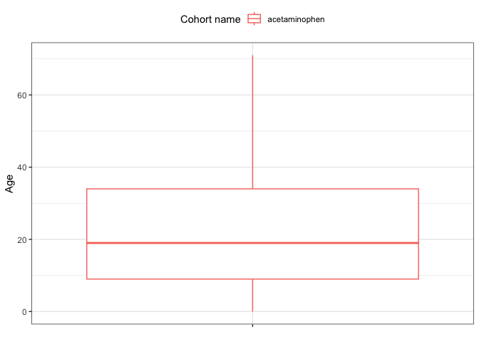
# Create a comparative boxplot of the age distribution across cohorts
plot_data <- dplyr::filter(chars, variable_name == "Age")
plotCharacteristics(plot_data, plotType = "boxplot", colour = "cohort_name")
Step 5: Advanced Characterization with Comorbidity Flags
The summariseCharacteristics function allows creating custom clinical flags with conceptIntersectFlag to assess pre-existing conditions in the baseline lookback window ($[-365, 0]$ days prior to cohort entry).
# Summarize baseline comorbidity flags in the 365 days prior to index
flags_summary <- cdm$nsaids |>
  summariseCharacteristics(
    demographics = FALSE,
    conceptIntersectFlag = list(
      "Baseline Comorbidities" = list(
        conceptSet = list(
          sinusitis = 4283893L,
          gi_bleed = 192671L,
          uti = 4116491L,
          asthma = 4051466L
        ),
        window = c(-365, 0)
      )
    )
  )

# Display the enriched characteristics table
tableCharacteristics(flags_summary)
| CDM name | ||||
|---|---|---|---|---|
| Synthea | ||||
| Variable name | Variable level | Estimate name | Cohort name | |
| celecoxib | diclofenac | |||
| Number records | – | N | 1,800 | 830 |
| Number subjects | – | N | 1,800 | 830 |
| Baseline comorbidities | Uti | N (%) | 7 (0.39%) | 4 (0.48%) |
| Sinusitis | N (%) | 19 (1.06%) | 4 (0.48%) | |
| Asthma | N (%) | 0 (0.00%) | 0 (0.00%) | |
| Gi bleed | N (%) | 0 (0.00%) | 0 (0.00%) | |