Impact Evaluation Studies Guide

Introduction & Purpose

Impact Evaluation Studies are a category of observational research designed to assess the real-world impact of large-scale “interventions” on population-level health outcomes or behaviours. These interventions are not assigned by a researcher (as in a clinical trial) but are typically external events such as new public health policies, regulatory actions, or changes in clinical guidelines.

The purpose of these studies is to determine whether a specific intervention caused a measurable change in trends. The central question is: “Did the intervention lead to a change in health outcomes or healthcare utilisation patterns at the population level?”

This methodology is crucial for evidence-based policymaking, allowing regulators and public health bodies to understand the real-world consequences of their decisions.

Study Designs

These studies are often called quasi-experimental because they aim to estimate a causal effect without the use of randomisation. The two most common designs in this category are:

1. Interrupted Time Series (ITS): This is the most common design. It involves tracking a population-level outcome over time, both before and after the intervention. The analysis then assesses whether the intervention was associated with a “break” or change in the trend of the outcome.
2. Difference-in-Differences (DiD): This design is used when the intervention affects one subpopulation but not another. It compares the change in the outcome trend in the “exposed” population to the change in the “unexposed” (control) population over the same period. This helps to control for other external factors that may have changed over time.

Participants

The study population is typically the entire source population or a large, relevant subset. For a DiD study, the population must be divisible into a group that was affected by the intervention and a group that was not.

Exposures

The “exposure” is the intervention itself. This is a discrete event that occurs at a specific, known point in time. Examples include:

• A new public health campaign (e.g., a smoking cessation campaign).
• A regulatory action, such as a drug safety warning or a Risk Minimisation Measure (RMM).
• A change in law or healthcare policy.

The study period is divided into a “pre-intervention” period and a “post-intervention” period.

Outcomes

The outcomes are population-level aggregate measures that are tracked over time. These can include:

• Incidence or prevalence rates of a disease.
• Rates of medication use.
• Hospitalisation rates.
• Rates of mortality.

Follow-up

The study involves a long-term follow-up of the population, typically spanning several years both before and after the intervention, to establish stable trends.

Analyses

The analysis uses statistical models to quantify the impact of the intervention.

• For ITS: A segmented regression model is used. This model fits a line to the pre-intervention trend and another line to the post-intervention trend. The analysis then tests for two things:
  1. A step change: An immediate jump or drop in the outcome level right after the intervention.
  2. A slope change: A change in the direction or steepness of the trend after the intervention.
• For DiD: A regression model is used to estimate the “difference in the differences,” which is the true causal effect of the intervention, having subtracted the background trend observed in the control group.

How to Implement This Study

Impact Evaluation Studies utilize quasi-experimental designs—such as Interrupted Time Series (ITS) and Difference-in-Differences (DiD)—to evaluate the causal impact of population-level health policies, regulatory safety warnings, or clinical guideline shifts on longitudinal disease rates or medication usage.

How Interrupted Time Series Works

• Longitudinal Rate Series: Tracking population-level incidence or prevalence rates over time across pre- and post-intervention periods.
• Intervention Threshold: A known calendar cutoff date (e.g. year of a regulatory risk minimization measure).
• Segmented Regression: Modeling the time series piecewise to test for:
  • Step Change ($\beta_2$): Immediate level jump or drop in outcome rate following the intervention.
  • Slope Change ($\beta_3$): Change in the long-term rate trajectory or gradient post-intervention.

Step 1: Setup & Connect to GiBleed

Load the required libraries and connect to the Eunomia GiBleed dataset using DuckDB:

library(CDMConnector)
library(CohortConstructor)
library(IncidencePrevalence)
library(visOmopResults)
library(dplyr)
library(ggplot2)
library(gt)

# Connect to Eunomia GiBleed dataset
Sys.setenv(EUNOMIA_DATA_FOLDER = Sys.getenv("EUNOMIA_DATA_FOLDER", tempdir()))
if (!eunomiaIsAvailable("GiBleed")) {
  downloadEunomiaData("GiBleed")
}

## 
## Download completed!

con <- DBI::dbConnect(duckdb::duckdb(), eunomiaDir("GiBleed"))
cdm <- cdmFromCon(con, cdmSchema = "main", writeSchema = "main")

Step 2: Define Outcome and Longitudinal Denominator

We track annual incidence rates of Gastrointestinal Hemorrhage (concept_id = 192671) across the source population observed from 1980 through 2019:

# 1. Instantiate Outcome Cohort
cdm$outcome <- conceptCohort(
  cdm = cdm,
  conceptSet = list(gi_bleed = 192671L),
  name = "outcome"
)

# 2. Instantiate Longitudinal Study Denominator
cdm <- generateDenominatorCohortSet(
  cdm = cdm,
  name = "denominator",
  cohortDateRange = as.Date(c("1980-01-01", "2019-01-01"))
)

Step 3: Estimate Longitudinal Incidence Rates

We calculate annual incidence rates per 100,000 person-years:

# Estimate annual incidence rates
inc <- estimateIncidence(
  cdm = cdm,
  denominatorTable = "denominator",
  outcomeTable = "outcome",
  interval = "years",
  outcomeWashout = Inf,
  repeatedEvents = FALSE
)

# Extract tidy rate table
rates_df <- visOmopResults::tidy(inc) |>
  filter(!is.na(incidence_100000_pys)) |>
  mutate(
    year = as.numeric(substr(incidence_start_date, 1, 4)),
    rate = as.numeric(incidence_100000_pys)
  ) |>
  arrange(year)

Step 4: Fit Segmented Regression (ITS Model)

We define a policy intervention threshold in the calendar year 2000 and construct the segmented time series variables:

# Set policy intervention year
intervention_year <- 2000

# Prepare segmented regression design matrix
its_df <- rates_df |>
  mutate(
    time = row_number(),
    post_int = ifelse(year >= intervention_year, 1, 0),
    time_after = ifelse(year >= intervention_year, year - intervention_year, 0)
  )

# Fit Segmented Linear Regression
its_model <- lm(rate ~ time + post_int + time_after, data = its_df)
its_df$fitted <- predict(its_model)

# Format regression coefficients
coefs <- summary(its_model)$coefficients
res_df <- data.frame(
  Parameter = c(
    "Baseline Intercept (Beta 0)",
    "Pre-intervention Slope (Beta 1)",
    "Immediate Step Change (Beta 2)",
    "Slope Change Post-intervention (Beta 3)"
  ),
  Estimate = round(coefs[, 1], 2),
  Std_Error = round(coefs[, 2], 2),
  t_value = round(coefs[, 3], 2),
  p_value = round(coefs[, 4], 4)
)

res_df |>
  gt() |>
  tab_header(
    title = "Segmented Regression Model Results",
    subtitle = "Impact Evaluation of Regulatory Warning (Year 2000)"
  ) |>
  cols_label(
    Parameter = "Model Parameter",
    Estimate = "Estimate",
    Std_Error = "Std. Error",
    t_value = "t-statistic",
    p_value = "p-value"
  )

Segmented Regression Model Results
Impact Evaluation of Regulatory Warning (Year 2000)
Model Parameter	Estimate	Std. Error	t-statistic	p-value
Baseline Intercept (Beta 0)	172.50	61.00	2.83	0.0077
Pre-intervention Slope (Beta 1)	15.00	5.09	2.95	0.0057
Immediate Step Change (Beta 2)	77.34	84.13	0.92	0.3642
Slope Change Post-intervention (Beta 3)	-13.17	7.50	-1.76	0.0876

Step 5: Plot Interrupted Time Series Trends

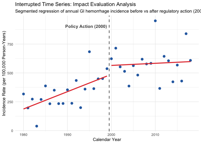
We plot the empirical annual rate estimates along with the segmented regression trajectories before and after the intervention:

ggplot(its_df, aes(x = year)) +
  geom_point(aes(y = rate), color = "#2b6cb0", size = 2.5) +
  geom_line(aes(y = fitted, group = post_int), color = "#e53e3e", linewidth = 1.2) +
  geom_vline(xintercept = intervention_year - 0.5, linetype = "dashed", color = "grey40", linewidth = 0.8) +
  annotate(
    "text",
    x = intervention_year - 1,
    y = max(its_df$rate) * 0.95,
    label = "Policy Action (2000)",
    hjust = 1,
    fontface = "bold",
    color = "grey30"
  ) +
  labs(
    title = "Interrupted Time Series: Impact Evaluation Analysis",
    subtitle = "Segmented regression of annual GI hemorrhage incidence before vs after regulatory action (2000)",
    x = "Calendar Year",
    y = "Incidence Rate (per 100,000 Person-Years)"
  ) +
  theme_minimal()