Health Economics & HCRU (HEOR / HTA) Guide
Introduction & Purpose
Health Economics and Outcomes Research (HEOR) and Healthcare Resource Utilisation (HCRU) studies evaluate the clinical value, resource burden, and economic impact of healthcare interventions in real-world clinical practice. While clinical trials establish efficacy and safety in idealized conditions, health economic evaluations generate evidence needed by Health Technology Assessment (HTA) bodies (e.g., NICE, HAS, G-BA, TLV) and healthcare payers to determine reimbursement, pricing, and cost-effectiveness.
The central questions addressed by HEOR/HCRU studies include:
- Healthcare Resource Utilisation (HCRU): How often do patients in a target cohort utilize healthcare services (inpatient hospitalizations, emergency visits, outpatient consultations, and pharmacotherapy)?
- Direct Medical Costs: What are the total and category-specific medical expenditures associated with managing a disease or treatment arm?
- Comparative Cost-Effectiveness: Is a new therapy cost-effective compared to the standard of care? What is the Incremental Cost-Effectiveness Ratio (ICER) per Quality-Adjusted Life Year (QALY) gained?
- Decision Uncertainty: What is the probability that the intervention is cost-effective at various Willingness-to-Pay (WTP) thresholds?
Study Design
HEOR studies typically employ a comparative longitudinal cohort design combined with decision-analytic Markov state-transition modeling. The design links real-world clinical encounters, medication dispenses, and financial cost records to simulate long-term economic trajectories.
Participants
The study defines two or more cohorts:
- Target Cohort: Patients initiating the intervention of interest (e.g., a novel therapeutic agent).
- Comparator Cohort: Patients initiating an alternative treatment or the standard of care.
Both cohorts require a baseline lookback period (e.g., 365 days of prior observation) to characterize demographic variables, comorbidities, and baseline resource utilization for causal adjustment.
Exposures & Comparators
- Target Exposure: The intervention or new technology being evaluated.
- Comparator Exposure: The active comparator or routine clinical standard of care.
Health Economic Endpoints & Resource Domains
Outcomes encompass both clinical events and economic resource consumption:
- HCRU Resource Domains:
- Inpatient & Critical Care: Hospital admissions, ICU stays, length of stay (LOS), and 30-/90-day readmissions.
- Outpatient & Ambulatory: Emergency room encounters, primary care visits, and specialist consultations.
- Pharmacotherapy: Medication fills, total days supply, and adherence/persistence (e.g., Proportion of Days Covered [PDC]).
- Procedures & Diagnostics: Surgical interventions, diagnostic imaging, and laboratory testing volumes.
- Post-Acute Care: Skilled nursing facility (SNF), rehabilitation, and home health services.
- Financial Expenditures: Direct medical costs extracted directly from the OMOP
costandvisit_occurrencetables (e.g.,total_paid,total_charge). - Health State Utilities & QALYs: Health-related quality of life weights mapped to disease states (e.g., progression-free survival vs. post-progression state).
Follow-up & Time Horizon
- Within-Trial / Observation Window: Empirical follow-up from the index date through available data to calculate observed HCRU rates and direct costs.
- Decision-Analytic Time Horizon: Long-term or lifetime horizon modeled using Markov state-transition simulations, with future costs and benefits discounted (typically 3%–5% annually).
Analyses
The analytical framework combines causal inference and health economic simulation:
- Baseline Characterisation & HCRU Extraction: Summarise demographics, clinical history, and baseline utilization across all resource categories.
- Causal Propensity Score Adjustment: Mitigate confounding by indication between treatment and comparator arms using regularized logistic regression (e.g., via
Cyclops) and greedy caliper matching or inverse probability of treatment weighting (IPTW). - State-Transition & Cost Modeling: Partition patient longitudinal journeys into discrete health state trajectories to estimate transition probability matrices and parametric cost distributions (e.g., Gamma or Log-Normal distributions).
- Probabilistic Sensitivity Analysis (PSA): Execute Monte Carlo simulations sampling transition rates, state costs, and utility values to capture parameter uncertainty.
- Decision Analysis (CEA): Calculate key HTA metrics:
- Incremental Cost-Effectiveness Ratio (ICER): $\Delta \text{Cost} / \Delta \text{QALY}$.
- Net Monetary Benefit (NMB): $\text{NMB}(k) = k \cdot \Delta E - \Delta C$ at willingness-to-pay threshold $k$.
- Visualizations: Cost-Effectiveness Acceptability Curves (CEAC) and Cost-Effectiveness Planes.
How to Implement This Study
The CohortEconomics, CohortUtilisation, and CohortCosts packages provide an end-to-end analytical framework for Health Economics and Outcomes Research (HEOR), Healthcare Resource Utilisation (HCRU) evaluation, and Health Technology Assessment (HTA) decision-analytic modeling directly from OMOP CDM databases.
How the 6-Stage HEOR Pipeline Works
- Study Initialisation & Baseline Characterisation: Defines comparative intervention arms and extracts demographic profiles.
- HCRU Extraction: Measures encounter rates and lengths of stay across inpatient admissions, emergency visits, outpatient consultations, pharmacotherapy, and procedures.
- Causal Propensity Score Adjustment: Adjusts for confounding by indication via regularized logistic regression and greedy caliper matching.
- Trajectory Compilation: Translates longitudinal patient clinical journeys into discrete Markov state-transition matrices.
- Economic Simulation (Markov PSA): Executes probabilistic sensitivity analysis sampling Gamma cost distributions and Beta health state utility weights over a defined time horizon.
- Decision Analysis (CEA): Estimates the Incremental Cost-Effectiveness Ratio (ICER), Net Monetary Benefit (NMB), Cost-Effectiveness Acceptability Curves (CEAC), and Cost-Effectiveness Planes.
Step 1: Setup & Connect to GiBleed
Load the necessary libraries and establish a connection to the Eunomia GiBleed dataset using DuckDB:
library(CohortEconomics)
library(CohortUtilisation)
library(CohortCosts)
library(CDMConnector)
library(CohortConstructor)
library(dplyr)
library(gt)
library(ggplot2)
# Connect to Eunomia GiBleed dataset
Sys.setenv(EUNOMIA_DATA_FOLDER = Sys.getenv("EUNOMIA_DATA_FOLDER", tempdir()))
if (!eunomiaIsAvailable("GiBleed")) {
  downloadEunomiaData("GiBleed")
}
##
## Download completed!
con <- DBI::dbConnect(duckdb::duckdb(), eunomiaDir("GiBleed"))
cdm <- cdmFromCon(con, cdmSchema = "main", writeSchema = "main")
Step 2: Define Target, Comparator, and Safety Outcome Cohorts
We instantiate new users of Celecoxib (concept_id = 1118084) as the target intervention, new users of Diclofenac (concept_id = 1124300) as the active comparator, and incident Gastrointestinal Hemorrhage (concept_id = 192671) as the primary health economic outcome:
# Target Cohort: Celecoxib new users
cdm$target_cohort <- conceptCohort(
  cdm = cdm,
  conceptSet = list(celecoxib = 1118084L),
  name = "target_cohort"
) |>
  requireIsFirstEntry()

# Comparator Cohort: Diclofenac new users
cdm$comparator_cohort <- conceptCohort(
  cdm = cdm,
  conceptSet = list(diclofenac = 1124300L),
  name = "comparator_cohort"
) |>
  requireIsFirstEntry()

# Outcome Cohort: Gastrointestinal Hemorrhage
cdm$outcome_cohort <- conceptCohort(
  cdm = cdm,
  conceptSet = list(gi_bleed = 192671L),
  name = "outcome_cohort"
)
Step 3: Baseline Characterisation & HCRU Extraction
We initialize the study, characterize baseline demographics, and extract longitudinal healthcare resource utilization across baseline ($[-365, -1]$ days) and follow-up ($[0, 365]$ days) windows:
# Initialize HEOR study and extract HCRU
study <- init(
  cdm = cdm,
  target_cohort = "target_cohort",
  comparator_cohort = "comparator_cohort",
  outcome_cohort = "outcome_cohort"
) |>
  summarise_baseline() |>
  extract_hcru(
    baseline_window = c(-365, -1),
    followup_window = c(0, 365)
  )

# Summarise per-patient resource utilization rates
hcru_summary <- study$hcru$patient_summary |>
  group_by(window) |>
  summarise(
    Mean_Inpatient_Admissions = round(mean(inpatient_admissions), 2),
    Mean_Inpatient_LOS_Days = round(mean(inpatient_los_days), 2),
    Mean_Prescription_Fills = round(mean(prescription_fills), 2),
    Mean_Procedure_Count = round(mean(procedure_count), 2),
    .groups = "drop"
  )

hcru_summary |>
  gt() |>
  tab_header(
    title = "Healthcare Resource Utilisation (HCRU) Summary",
    subtitle = "Resource Consumption Across Baseline vs Follow-up Windows"
  ) |>
  cols_label(
    window = "Observation Window",
    Mean_Inpatient_Admissions = "Inpatient Admissions (Mean)",
    Mean_Inpatient_LOS_Days = "Length of Stay Days (Mean)",
    Mean_Prescription_Fills = "Prescription Fills (Mean)",
    Mean_Procedure_Count = "Procedures & Tests (Mean)"
  )
| Healthcare Resource Utilisation (HCRU) Summary | ||||
| Resource Consumption Across Baseline vs Follow-up Windows | ||||
| Observation Window | Inpatient Admissions (Mean) | Length of Stay Days (Mean) | Prescription Fills (Mean) | Procedures & Tests (Mean) |
|---|---|---|---|---|
| baseline | 0.00 | 0.00 | 0.33 | 0.21 |
| followup | 0.19 | 0.19 | 1.35 | 0.21 |
Step 4: Causal Propensity Score Matching & Trajectory Compilation
We fit a regularized logistic regression propensity score model, perform 1:1 nearest-neighbor matching, and compile Markov state-transition probability matrices:
# Causal propensity score adjustment and discrete trajectory modeling
study <- study |>
  fit_ps() |>
  adjust_ps(caliper = 0.2) |>
  compile_trajectories()

# Assign parametric state-specific unit costs (Baseline maintenance vs GI Bleed event)
study$costs <- data.frame(
  health_state = c("State_Baseline", "State_Outcome"),
  mean_cost = c(450, 4800),
  se_cost = c(40, 350)
)
Step 5: Economic Simulation (Markov PSA) & Cost-Effectiveness Analysis
We execute a 10-year Monte Carlo Probabilistic Sensitivity Analysis (PSA) with 3% annual discounting, followed by decision analysis:
# Execute Probabilistic Sensitivity Analysis simulation
sim <- simulate_economics(
  traj_obj = study,
  time_horizon = 10,
  discount_rate = 0.03,
  n_samples = 250
)

# Run Cost-Effectiveness Decision Analysis
cea <- run_cea(sim)
Step 6: HTA Decision Plots (CEAC & Cost-Effectiveness Plane)
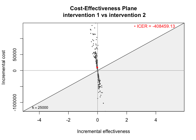
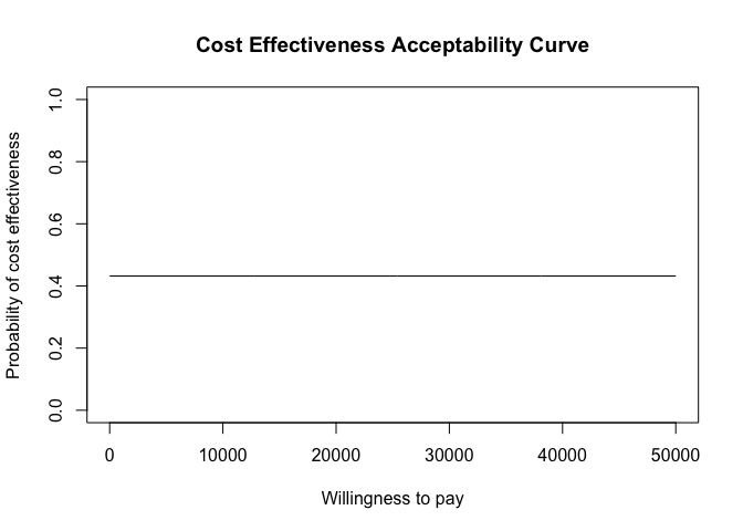
We generate the Cost-Effectiveness Acceptability Curve (CEAC) showing the probability of cost-effectiveness across Willingness-to-Pay thresholds, and the Cost-Effectiveness Plane:
# Plot Cost-Effectiveness Acceptability Curve (CEAC)
plot_ceac(cea)
# Plot Cost-Effectiveness Plane
plot_plane(cea)