Drug Utilisation Guide
Introduction & Purpose
Drug Utilisation Studies (DUS) are designed to investigate how medicines are used in real-world clinical practice. While clinical trials tell us if a drug can work in a controlled setting, DUS tells us how it is actually being used by the general population. This is crucial for understanding prescribing patterns, patient adherence, and the real-world context of medication use.
The purpose of a DUS can be broad, but it often focuses on answering questions like:
- How many people are using a specific drug?
- For what medical reasons (indications) is it being prescribed?
- What is the typical starting dose?
- How long do patients typically remain on the treatment (persistence)?
- Are there specific populations who are more likely to use the drug?
Study Design
DUS can be conducted at two different levels, and a comprehensive study often includes both:
- Population-Level DUS: A descriptive analysis of drug use across an entire population.
- Patient-Level DUS: A cohort study focusing on the characteristics and behaviours of individuals who initiate a specific drug.
Participants
- For Population-Level DUS: The study includes the entire source population available in the database.
- For Patient-Level DUS: The study includes a cohort of new users of a specific drug or drug class. A “washout” period (e.g., one year with no prior use) is required to ensure that the individuals are genuinely new users. The cohort can also be restricted to a subpopulation of interest (e.g., only patients with a prior diagnosis of a specific condition).
Exposures
The primary “exposure” of interest is the medication itself. The analysis can focus on a single drug, a class of drugs, or compare the usage patterns of multiple drugs.
Outcomes
The outcomes in a DUS are measures of medication usage. These can include:
- At the Population Level:
- Incidence of Use: The rate of new users of a drug over time.
- Prevalence of Use: The proportion of the population using a drug at a specific point in time.
- At the Patient Level:
- Initial Dose: The dose prescribed at the start of treatment.
- Treatment Duration: The length of time a patient remains on the drug.
- Treatment Discontinuation & Switching: How often patients stop the drug or switch to another.
- Patient Characteristics: A baseline characterisation of the new users.
Follow-up
- For Population-Level DUS: Follow-up is typically over calendar time to assess trends in usage.
- For Patient-Level DUS: Follow-up starts on the date of therapy initiation (the index date) and continues until the end of data availability, loss to follow-up, or a pre-defined study end date.
Analyses
The analysis is primarily descriptive.
- Population-level analyses mirror those in an epidemiology study: calculating the incidence and prevalence of use, often stratified by age, gender, and calendar year.
- Patient-level analyses involve characterising the new user cohort and summarising the key usage metrics, such as median treatment duration and the distribution of initial doses.
How to Implement This Study
The DrugUtilisation package provides standardized workflows to characterize real-world prescription patterns, treatment duration, dosage, indications, and longitudinal medication adherence from OMOP CDM databases.
How DrugUtilisation works
- New-User Cohorts: Generate drug exposure cohorts with customizable washout and prior observation criteria using
CohortConstructor. - Utilisation Metrics: Calculate cumulative exposure duration, number of treatment eras, and quantity using
summariseDrugUtilisation(). - Indication Analysis: Identify recorded clinical diagnoses prior to therapy initiation using
summariseIndication(). - Adherence & Persistence: Measure treatment continuity via Proportion of Patients Covered (PPC) curves using
summariseProportionOfPatientsCovered().
Step 1: Setup & Connect to GiBleed
First, load the required libraries and establish a connection to the Eunomia GiBleed dataset using DuckDB:
library(CDMConnector)
library(CohortConstructor)
library(DrugUtilisation)
library(visOmopResults)
library(dplyr)
# Connect to Eunomia GiBleed dataset
Sys.setenv(EUNOMIA_DATA_FOLDER = Sys.getenv("EUNOMIA_DATA_FOLDER", tempdir()))
if (!eunomiaIsAvailable("GiBleed")) {
  downloadEunomiaData("GiBleed")
}
##
## Download completed!
con <- DBI::dbConnect(duckdb::duckdb(), eunomiaDir("GiBleed"))
cdm <- cdmFromCon(con, cdmSchema = "main", writeSchema = "main")
Step 2: Define New-User Drug Cohort
We define a cohort of new users of Celecoxib (concept_id = 1118084) with at least 365 days of prior observation:
# Create new-user Celecoxib cohort with 365 days prior observation
cdm$celecoxib <- conceptCohort(
  cdm = cdm,
  conceptSet = list(celecoxib = 1118084L),
  name = "celecoxib"
) |>
  requireIsFirstEntry() |>
  requirePriorObservation(minPriorObservation = 365)
Step 3: Summarise Drug Utilisation Metrics
We calculate key utilisation metrics including duration of exposure, number of eras, and cumulative quantity:
# Summarise drug utilisation metrics
dus_summary <- cdm$celecoxib |>
  summariseDrugUtilisation(
    ingredientConceptId = 1118084L
  )

# Display publication table
tableDrugUtilisation(dus_summary)
| Concept set | Variable name | Estimate name | Data source |
|---|---|---|---|
| Synthea | |||
| celecoxib | |||
| overall | number records | N | 1,800 |
| number subjects | N | 1,800 | |
| ingredient_1118084_descendants | number exposures | missing N (%) | 0 (0.00 %) |
| Mean (SD) | 1.00 (0.00) | ||
| Median (Q25 - Q75) | 1 (1 - 1) | ||
| time to exposure | missing N (%) | 0 (0.00 %) | |
| Mean (SD) | 0.00 (0.00) | ||
| Median (Q25 - Q75) | 0 (0 - 0) | ||
| cumulative quantity | missing N (%) | 0 (0.00 %) | |
| Mean (SD) | 0.00 (0.00) | ||
| Median (Q25 - Q75) | 0.00 (0.00 - 0.00) | ||
| initial quantity | missing N (%) | 0 (0.00 %) | |
| Mean (SD) | 0.00 (0.00) | ||
| Median (Q25 - Q75) | 0.00 (0.00 - 0.00) | ||
| initial exposure duration | missing N (%) | 0 (0.00 %) | |
| Mean (SD) | 1.00 (0.00) | ||
| Median (Q25 - Q75) | 1 (1 - 1) | ||
| number eras | missing N (%) | 0 (0.00 %) | |
| Mean (SD) | 1.00 (0.00) | ||
| Median (Q25 - Q75) | 1 (1 - 1) | ||
| days exposed | missing N (%) | 0 (0.00 %) | |
| Mean (SD) | 1.00 (0.00) | ||
| Median (Q25 - Q75) | 1 (1 - 1) | ||
| days prescribed | missing N (%) | 0 (0.00 %) | |
| Mean (SD) | 1.00 (0.00) | ||
| Median (Q25 - Q75) | 1 (1 - 1) | ||
Step 4: Indication Profiling
We profile baseline clinical indications (such as acute sinusitis, UTI, and asthma) recorded in the 365-day and 30-day windows prior to drug initiation:
# Define potential indication cohorts
cdm$indications <- conceptCohort(
  cdm = cdm,
  conceptSet = list(
    sinusitis = 4283893L,
    uti = 4116491L,
    asthma = 4051466L
  ),
  name = "indications"
)

# Summarise indications prior to treatment start
ind_summary <- cdm$celecoxib |>
  summariseIndication(
    indicationCohortName = "indications",
    indicationWindow = list(c(-365, 0), c(-30, 0))
  )

# Display indication table
tableIndication(ind_summary)
| Data source | ||
|---|---|---|
| Synthea | ||
| Indication | Estimate name | Cohort name |
| celecoxib | ||
| Indication from 365 days before to the index date | ||
| asthma | N (%) | 0 (0.00 %) |
| sinusitis | N (%) | 19 (1.06 %) |
| uti | N (%) | 7 (0.39 %) |
| asthma and sinusitis | N (%) | 0 (0.00 %) |
| asthma and uti | N (%) | 0 (0.00 %) |
| sinusitis and uti | N (%) | 0 (0.00 %) |
| asthma and sinusitis and uti | N (%) | 0 (0.00 %) |
| none | N (%) | 1,774 (98.56 %) |
| not in observation | N (%) | 0 (0.00 %) |
| Indication from 30 days before to the index date | ||
| asthma | N (%) | 0 (0.00 %) |
| sinusitis | N (%) | 4 (0.22 %) |
| uti | N (%) | 2 (0.11 %) |
| asthma and sinusitis | N (%) | 0 (0.00 %) |
| asthma and uti | N (%) | 0 (0.00 %) |
| sinusitis and uti | N (%) | 0 (0.00 %) |
| asthma and sinusitis and uti | N (%) | 0 (0.00 %) |
| none | N (%) | 1,794 (99.67 %) |
| not in observation | N (%) | 0 (0.00 %) |
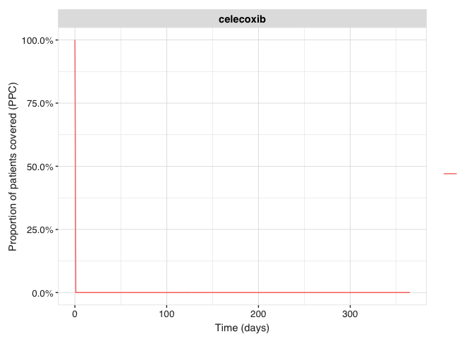
Step 5: Proportion of Patients Covered (Adherence)
We compute and visualize the Proportion of Patients Covered (PPC) over a 365-day post-index horizon to examine longitudinal treatment persistence:
# Calculate PPC over 365 days of follow-up
ppc <- cdm$celecoxib |>
  summariseProportionOfPatientsCovered(
    followUpDays = 365
  )

# Plot longitudinal patient coverage curve
plotProportionOfPatientsCovered(ppc)